Topic 2: Functions

IB DP MATHEMATICS Analysis and Approaches (AA) Topic 2 Functions

Revision Notes · Standard and Higher Level Fahad H. Ahmad

+92 323 509 4443 | Megalecture.com

Original notes prepared for the IB Diploma Programme Mathematics: Analysis and Approaches course (first assessment 2021)

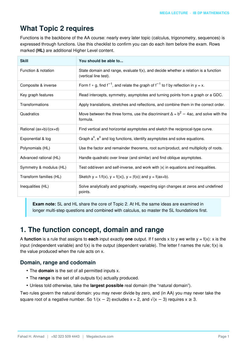
What Topic 2 requires

Functions is the backbone of the AA course: nearly every later topic (calculus, trigonometry, sequences) is expressed through functions. Use this checklist to confirm you can do each item before the exam. Rows marked (HL) are additional Higher Level content.

Skill You should be able to...

Function & notation State domain and range, evaluate f(x), and decide whether a relation is a function (vertical line test).

Composite & inverse Form f ∘ g, find f−1, and relate the graph of f−1 to f by reflection in y = x.

Key graph features Read intercepts, symmetry, asymptotes and turning points from a graph or a GDC.

Transformations Apply translations, stretches and reflections, and combine them in the correct order.

Quadratics Move between the three forms, use the discriminant Δ = b2 − 4ac, and solve with the formula.

Rational (ax+b)/(cx+d) Find vertical and horizontal asymptotes and sketch the reciprocal-type curve.

Exponential & log Graph ax, ex and log functions, identify asymptotes and solve equations.

Polynomials (HL) Use the factor and remainder theorems, root sum/product, and multiplicity of roots.

Advanced rational (HL) Handle quadratic over linear (and similar) and find oblique asymptotes.

Symmetry & modulus (HL) Test odd/even and self-inverse, and work with |x| in equations and inequalities.

Transform families (HL) Sketch y = 1/f(x), y = f(|x|), y = |f(x)| and y = f(ax+b).

Inequalities (HL) Solve analytically and graphically, respecting sign changes at zeros and undefined points.

Exam note: SL and HL share the core of Topic 2. At HL the same ideas are examined in longer multi-step questions and combined with calculus, so master the SL foundations first.

1. The function concept, domain and range

A function is a rule that assigns to each input exactly one output. If f sends x to y we write y = f(x): x is the input (independent variable) and f(x) is the output (dependent variable). The letter f names the rule; f(x) is the value produced when the rule acts on x.

Domain, range and codomain

• The domain is the set of all permitted inputs x.
• The range is the set of all outputs f(x) actually produced.
• Unless told otherwise, take the largest possible real domain (the “natural domain”).

Two rules govern the natural domain: you may never divide by zero, and (in AA) you may never take the square root of a negative number. So 1/(x − 2) excludes x = 2, and √(x − 3) requires x ≥ 3.

Function Natural domain Range f(x) = x2 x ∈ ℝ f(x) ≥ 0 f(x) = √x x ≥ 0 f(x) ≥ 0 f(x) = 1/x x ≠ 0 f(x) ≠ 0 f(x) = 2x x ∈ ℝ f(x) > 0 f(x) = ln x x > 0 f(x) ∈ ℝ

Mappings and the vertical line test

A relation is a function only if every input has a single output. Graphically this is the vertical line test: any vertical line meets the graph at most once. A circle x2 + y2 = 9 fails the test, so it is not a function of x. Mappings are also classified by how inputs pair with outputs:

• one-to-one: different inputs give different outputs (e.g. f(x) = 2x + 1).
• many-to-one: different inputs can share an output (e.g. f(x) = x2, since 3 and −3 both map to 9).

Why it matters: Only one-to-one functions have an inverse over their whole domain. A many-to-one function must first have its domain restricted before it can be inverted (see Section 2).

2. Composite and inverse functions

Composite functions

A composite applies one function to the output of another. (f ∘ g)(x) = f(g(x)) means “do g first, then f”. Work from the inside out. Order matters: in general f ∘ g ≠ g ∘ f.

The composite g(x) must land inside the domain of f. So the domain of f ∘ g is the set of x in the domain of g for which g(x) lies in the domain of f.

Worked example 1 - composite and inverse

Let f(x) = 2x + 3 and g(x) = x2. Find (a) (f ∘ g)(x), (b) (g ∘ f)(x), (c) f−1(x).

• (f ∘ g)(x) = f(x2) = 2x2 + 3.
• (g ∘ f)(x) = g(2x + 3) = (2x + 3)2 = 4x2 + 12x + 9.

Parts (a) and (b) differ, confirming the order of composition matters.

• Write y = 2x + 3, swap the roles and solve for x: x = (y − 3)/2, so f−1(x) = (x − 3)/2. Check: f(f−1(x)) = 2 × (x − 3)/2 + 3 = x.

Inverse functions

The inverse f−1 reverses f: if f(a) = b then f−1(b) = a. It exists only when f is one-to-one. Key relationships:

• f−1(f(x)) = x and f(f−1(x)) = x on the appropriate domains.
• domain of f−1 = range of f, and range of f−1 = domain of f.
• the graph of y = f−1(x) is the reflection of y = f(x) in the line y = x; every point (a, b) becomes (b, a).

Method to find an inverse: (1) write y = f(x); (2) interchange x and y; (3) solve for y; (4) rename the result f−1(x); (5) state its domain (= the range of f). The −1 notation means the inverse, not the reciprocal 1/f.

Common pitfall: For f(x) = x2 there is no inverse over all of ℝ because it is many-to-one. Restrict the domain, e.g. to x ≥ 0, giving f−1(x) = √x with domain x ≥ 0.

3. Graphing functions and their key features

When you sketch or analyse a graph, examiners expect you to label the same short list of features every time.

Feature How to find it What it looks like y-intercept Evaluate f(0) where the curve crosses the y-axis x-intercept(s) / zeros Solve f(x) = 0 where the curve crosses the x-axis

Vertical asymptote Input value where f is undefined (denominator = 0) curve shoots to ±∞ near a vertical line

Horizontal asymptote Behaviour as x → ±∞ curve levels off toward a horizontal line

Maximum / minimum Turning points (GDC or completing the square) local peak or valley of the curve

Symmetry Even: f(−x) = f(x); odd: f(−x) = −f(x) mirror in y-axis / rotational about O

An asymptote is a line the curve approaches arbitrarily closely but never reaches. A graph may cross a horizontal asymptote in its middle region; what matters is the behaviour far out, as x → ±∞.

GDC habit: Set a sensible window, then use the built-in tools for zeros, intersections and maxima/minima rather than reading pixels by eye. Always quote GDC answers to 3 significant figures unless told otherwise.

4. Transformations of graphs

Starting from y = f(x), each algebraic change produces a predictable geometric change. Split them into changes outside f (they affect y, and behave the “obvious” way) and changes inside f (they affect x, and behave the opposite way to what you might expect).

Transformation Effect on the graph Effect on a point (x, y) y = f(x) + b translation b units up (down if b < 0) (x, y + b) y = f(x − a) translation a units right (left if a < 0) (x + a, y) y = a f(x) vertical stretch, scale factor a (x, a y) y = f(x/a) or f(bx) horizontal stretch, factor a = 1/b (a x, y) y = −f(x) reflection in the x-axis (x, −y)

Transformation Effect on the graph Effect on a point (x, y) y = f(−x) reflection in the y-axis (−x, y)

Figure 1. Transformations of y = x2. The dashed curves are y = (x − 2)2 + 1 (translation 2 right and 1 up, vertex (2, 1)) and y =

−2x2 (reflection in the x-axis with vertical stretch factor 2).

Combining transformations - order matters

For a chain such as y = a f(b(x − h)) + k, apply horizontal operations in the reverse of the usual algebra order, then vertical operations. A safe recipe: horizontal translation and stretch first (inside the bracket, working on x), then vertical stretch/reflection, then vertical translation last. Vertical and horizontal families are independent, so a vertical stretch followed by a horizontal shift can be done in either order relative to each other.

Worked example 2 - tracking a point through transformations

The graph of y = f(x) passes through the point (2, 5). Find the image of this point on (a) y = 3f(x −

• − 4 and (b) y = f(2x).
• The bracket x − 1 must equal 2, so x = 3. Then y = 3(5) − 4 = 11. Image: (3, 11).
• Here 2x must equal 2, so x = 1, and the output is unchanged: y = 5. Image: (1, 5) - a horizontal stretch of factor 1/2.

Notice the inside change (x − 1, 2x) acts on the x-coordinate in the opposite sense to intuition, while 3(...) − 4 acts directly on y.

Common pitfall: y = f(2x) is a horizontal stretch of factor 1/2 (a squeeze), not a stretch by 2. Inside changes always invert.

5. Quadratic functions

A quadratic f(x) = ax2 + bx + c (a ≠ 0) has a parabola graph, opening up if a > 0 and down if a < 0. The same quadratic can be written three ways, each revealing something different.

Form Written as Reveals

Standard ax2 + bx + c y-intercept c

Completed square / vertex a(x − h)2 + k vertex (h, k); axis x = h

Factored a(x − p)(x − q) x-intercepts p and q

The axis of symmetry is x = −b/(2a); the vertex lies on it. The vertex is the minimum point when a > 0 and the maximum point when a < 0. Completing the square converts standard form to vertex form and is the exam's preferred way to find the turning point by hand.

Figure 2. Key features of y = x2 − 2x − 3. Roots (−1, 0) and (3, 0), vertex (1, −4), axis of symmetry x = 1 (dashed) and y-intercept (0, −3).

Worked example 3 - completing the square

Express f(x) = 2x2 − 12x + 7 in vertex form and state the coordinates and nature of the turning point.

Take the factor 2 from the x-terms: f(x) = 2(x2 − 6x) + 7.

Complete the square inside: x2 − 6x = (x − 3)2 − 9.

So f(x) = 2[(x − 3)2 − 9] + 7 = 2(x − 3)2 − 18 + 7 = 2(x − 3)2 − 11.

Vertex (3, −11); since a = 2 > 0 it is a minimum; axis x = 3; minimum value f(3) = −11.

The discriminant and nature of the roots

For ax2 + bx + c = 0 the roots come from the quadratic formula x = ( −b ± √(b2 − 4ac) ) / (2a)

The quantity under the root, Δ = b2 − 4ac, is the discriminant. It decides how many real roots there are without solving.

Discriminant Real roots Graph meets x-axis

Δ > 0 two distinct real roots at two points

Δ = 0 one repeated (double) root touches at the vertex

Δ < 0 no real roots does not cross the axis

Worked example 4 - using the discriminant

Find the values of k for which 2x2 + kx + 8 = 0 has (a) equal roots, (b) two distinct real roots.

Here a = 2, b = k, c = 8, so Δ = k2 − 4(2)(8) = k2 − 64.

• Equal roots need Δ = 0: k2 = 64, so k = ±8.
• Two distinct real roots need Δ > 0: k2 > 64, so k > 8 or k < −8.

Common pitfall: Δ = 0 gives one (repeated) root, not zero roots. “No real roots” is Δ < 0. Read the wording carefully: “equal roots” and “tangent to the x-axis” both mean Δ = 0.

6. Reciprocal and simple rational functions

The reciprocal function f(x) = 1/x has a rectangular hyperbola graph with two branches. Its domain is x ≠ 0 and its range is f(x) ≠ 0; the axes are its asymptotes: the vertical asymptote is x = 0 and the horizontal asymptote is y = 0. It is an odd function, symmetric under a half-turn about the origin.

The general linear-over-linear function

f(x) = (ax + b)/(cx + d) has the same hyperbola shape, shifted. Its asymptotes come from two simple rules:

• Vertical asymptote: where the denominator is zero, x = −d/c.
• Horizontal asymptote: the ratio of the leading coefficients, y = a/c (the limiting value as x → ±∞).
• x-intercept: where the numerator is zero, x = −b/a; y-intercept: f(0) = b/d.

Worked example 5 - asymptotes of a rational function

Sketch the key features of f(x) = (3x − 2)/(x + 1).

Vertical asymptote: x + 1 = 0, so x = −1.

Horizontal asymptote: leading coefficients 3 and 1, so y = 3.

x-intercept: 3x − 2 = 0, so x = 2/3. y-intercept: f(0) = −2/1 = −2.

The curve has two branches sitting either side of x = −1 and approaching y = 3 far from the origin.

Figure 3. y = 1/(x − 2) + 1 has a vertical asymptote x = 2 and a horizontal asymptote y = 1 (both dashed); the x-intercept is (1,

• and the y-intercept is (0, 0.5).

7. Exponential and logarithmic functions

An exponential function f(x) = ax (a > 0, a ≠ 1) has domain ℝ and range f(x) > 0. Every such graph passes through (0, 1), rises if a > 1 and falls if 0 < a < 1, and has the x-axis (y = 0) as a horizontal asymptote. The special base e ≈ 2.718 gives the natural exponential ex.

A logarithmic function f(x) = loga x is the inverse of ax. Its domain is x > 0 and its range is ℝ; it passes through (1, 0) and has the y-axis (x = 0) as a vertical asymptote. Because they are inverses, the graphs of ax and loga x are reflections of each other in y = x. The natural logarithm ln x = loge x.

Function Domain Range Asymptote Passes through ax (a > 1) x ∈ ℝ y > 0 y = 0 (0, 1) ex x ∈ ℝ y > 0 y = 0 (0, 1) loga x x > 0 y ∈ ℝ x = 0 (1, 0) ln x x > 0 y ∈ ℝ x = 0 (1, 0)

Figure 4. y = ex and its inverse y = ln x are reflections of each other in the line y = x (dashed). They pass through (0, 1) and (1,

• respectively.

Solving equations: use that ax = b means x = loga b, and that ln and ex undo each other. For example, 2 × 3x = 54 gives 3x = 27, so x = 3; and ex = 10 gives x = ln 10 ≈ 2.30.

Domain alert: log and ln accept only positive inputs. After solving a log equation, reject any solution that would make the argument zero or negative - a routine source of lost marks.

8. Solving equations graphically and with the GDC

Any equation g(x) = h(x) can be solved by graphing y = g(x) and y = h(x) and reading the x-coordinates of their intersection points; equivalently, graph y = g(x) − h(x) and find its zeros. This is essential when no exact algebraic method exists, for instance ex = 3 − x.

• Choose a viewing window that shows all intersections you expect.
• Use the GDC's intersect or zero tools, not tracing by eye.
• Report each solution to 3 significant figures unless an exact value is asked for, and check none has been missed by scanning the whole relevant range.

Exam technique: On a calculator paper, a quick GDC sketch confirms how many solutions an equation has before you commit to an algebraic route - and can rescue full marks when the algebra stalls.

9. Polynomial functions (HL)

A polynomial of degree n has the form anxn + ... + a1x + a0. Two theorems make factorising and root-finding efficient.

• Remainder theorem: the remainder when p(x) is divided by (x − a) equals p(a).
• Factor theorem: (x − a) is a factor of p(x) exactly when p(a) = 0. (More generally (bx − a) is a factor when p(a/b) = 0.)

Sum and product of roots

For a polynomial anxn + ... + a0 with roots r1, ..., rn, the sum of the roots is −an−1/an and the product of the roots is (−1)n a0/an. For a quadratic ax2 + bx + c: sum = −b/a and product = c/a.

Multiplicity and the shape of the graph

If (x − a)m divides p(x) exactly, then a is a root of multiplicity m. At a root of odd multiplicity the curve crosses the x-axis; at a root of even multiplicity it touches and turns back. A double root (m = 2) sits at a turning point on the axis.

Worked example 6 - factor and remainder theorems (HL)

For p(x) = 2x3 − 3x2 − 11x + 6, (a) show (x − 3) is a factor, (b) factor p(x) fully and state the roots,

• find the remainder when p(x) is divided by (x − 2).
• p(3) = 2(27) − 3(9) − 11(3) + 6 = 54 − 27 − 33 + 6 = 0, so by the factor theorem (x − 3) is a factor.
• Dividing gives p(x) = (x − 3)(2x2 + 3x − 2) = (x − 3)(2x − 1)(x + 2). Roots: x = 3, x = 1/2, x = −2.

Check by root sum: −b/a = 3/2, and 3 + 1/2 − 2 = 3/2.

• By the remainder theorem the remainder is p(2) = 16 − 12 − 22 + 6 = −12.

Figure 5. y = (x + 2)(x − 1)(x − 3) crosses the x-axis at its three real roots x = −2, 1 and 3; the y-intercept is (0, 6).

10. Rational functions and oblique asymptotes (HL)

At HL the numerator or denominator may be quadratic. Locate features as follows:

• Vertical asymptotes: values that make the denominator zero (and do not cancel with the numerator).
• Horizontal asymptote: if numerator and denominator have the same degree, y = ratio of leading coefficients; if the numerator degree is smaller, y = 0.
• Oblique (slant) asymptote: if the numerator degree is exactly one more than the denominator, polynomial division gives a straight line y = mx + c that the curve approaches as x → ±∞.

For example f(x) = (x2 + 1)/(x − 1) divides to x + 1 + 2/(x − 1). As x → ±∞ the fraction 2/(x − 1) → 0, so the oblique asymptote is y = x + 1, and the vertical asymptote is x = 1.

Method reminder: Find an oblique asymptote by long (or synthetic) division: the quotient is the asymptote line, and the leftover fraction tends to 0 far from the origin.

11. Odd, even and self-inverse functions (HL)

• Even: f(−x) = f(x) for all x. The graph is symmetric in the y-axis. Examples: x2, cos x, |x|.
• Odd: f(−x) = −f(x) for all x. The graph has rotational symmetry of order 2 about the origin. Examples: x3, sin x, 1/x.

Most functions are neither. To test, compute f(−x) and compare it with f(x) and −f(x).

Self-inverse functions

A function is self-inverse if f−1 = f, that is f(f(x)) = x for all x in the domain. Its graph is symmetric in the line y = x. Examples include f(x) = 1/x, f(x) = a − x, and f(x) = (x + b)/(x − 1) type hyperbolas for suitable constants. To verify, show f(f(x)) simplifies to x.

Quick check: For a self-inverse function, reflecting its graph in y = x leaves it unchanged - a fast visual confirmation on the GDC.

12. The modulus (absolute value) function (HL)

The modulus |x| gives the non-negative size of x: |x| = x when x ≥ 0 and |x| = −x when x < 0. The graph of y = |x| is a V with vertex at the origin; y = |x − a| has its vertex at (a, 0). Geometrically |x − a| is the distance between x and a on the number line.

Figure 6. y = |x − 1| is a V-shape with its vertex at (1, 0) and y-intercept (0, 1).

Solving modulus equations and inequalities

• |x| = k (k ≥ 0) means x = k or x = −k.
• |x| < k means −k < x < k (a single interval).
• |x| > k means x < −k or x > k (two pieces).
• |A| = |B| can be solved by squaring: A2 = B2.

Worked example 7 - modulus equation and inequality (HL)

Solve (a) |2x − 1| = |x + 3| and (b) |x − 2| < 3.

• Square both sides: (2x − 1)2 = (x + 3)2.

4x2 − 4x + 1 = x2 + 6x + 9, so 3x2 − 10x − 8 = 0.

Factor: (3x + 2)(x − 4) = 0, giving x = −2/3 or x = 4 (both check).

• |x − 2| < 3 means −3 < x − 2 < 3, so −1 < x < 5.

Common pitfall: Squaring is valid for |A| = |B| and |A| < |B| type statements because both sides are non-negative. Do not square |A| = B unless you have first checked B ≥ 0.

13. Graphs of related functions (HL)

Given the graph of y = f(x), you should be able to sketch four related graphs.

Graph How to build it from y = f(x) y = |f(x)| reflect every part below the x-axis up above it; parts already above stay put y = f(|x|) keep the graph for x ≥ 0, then reflect that part in the y-axis (the x < 0 side is discarded)

Graph How to build it from y = f(x) y = 1/f(x) zeros of f become vertical asymptotes; where f → ±∞, 1/f → 0; maxima of f become minima of 1/f and vice versa; the sign is preserved y = f(ax + b) a horizontal stretch of factor 1/a then a translation; treat it as f(a(x + b/a))

For y = 1/f(x), a useful anchor is that points where f(x) = 1 or f(x) = −1 are unchanged, since their reciprocal is the same value. Watch signs: 1/f keeps the sign of f, so it never jumps across an asymptote without f passing through zero.

Order matters: y = |f(x)| reflects outputs (in the x-axis) while y = f(|x|) reflects inputs (in the y-axis). They usually give different graphs - sketch both carefully.

14. Solving inequalities analytically and graphically (HL)

Inequalities are solved by finding where an expression changes sign. The sign can only change at a zero (numerator = 0) or at an undefined point (denominator = 0). Mark these critical values on a number line and test the sign of the expression in each interval.

• Never multiply both sides of an inequality by an expression that could be negative - the direction of the inequality may flip. Instead move everything to one side and analyse the sign of the single combined expression.
• Include a zero of the numerator when the sign is ≥ or ≤, but never include a value that makes the denominator zero.
• Graphically, solve f(x) > g(x) by reading where the graph of f lies above the graph of g.

Example: to solve (x − 1)/(x + 2) ≥ 0, the critical values are x = 1 (numerator zero) and x = −2 (denominator zero, excluded). Testing the three intervals gives the solution x < −2 or x ≥ 1.

Common pitfall: x = −2 is excluded even though the inequality is “greater than or equal to”, because the expression is undefined there. Use an open circle at excluded points and a filled circle at included zeros.

Quick reference

Idea Key result

Composite (f ∘ g)(x) = f(g(x)); order matters, f ∘ g ≠ g ∘ f

Inverse swap x and y then solve; domain f−1 = range f; reflect in y = x

Quadratic vertex a(x − h)2 + k has vertex (h, k), axis x = h = −b/(2a)

Quadratic formula x = ( −b ± √(b2 − 4ac) ) / (2a)

Discriminant Δ = b2 − 4ac: >0 two roots, =0 one, <0 none

(ax+b)/(cx+d) vertical x = −d/c; horizontal y = a/c

Exponential ax range y > 0; asymptote y = 0; through (0, 1)

Idea Key result

Logarithm loga x domain x > 0; asymptote x = 0; through (1, 0)

Factor theorem (HL) (x − a) factor of p(x) iff p(a) = 0

Oblique asymptote (HL) numerator degree one more than denominator; divide to find y = mx + c

Even / odd (HL) even f(−x) = f(x); odd f(−x) = −f(x)

Modulus (HL) |x| < k gives −k < x < k; |x| > k gives two pieces

Test yourself

Attempt all ten without notes, then check against the full solutions. Questions marked (HL) are Higher Level.

• For f(x) = 3x − 4 and g(x) = x2 + 1, find (f ∘ g)(2) and (g ∘ f)(x).
• Find the inverse of f(x) = (2x + 1)/(x − 3) and state its domain.
• Express f(x) = 3x2 + 12x + 5 in vertex form and state the minimum point.
• Find the values of m for which x2 − mx + 9 = 0 has two distinct real roots.
• Describe the transformations mapping y = x2 to y = −(x − 1)2 + 4 and state the vertex.
• State the vertical and horizontal asymptotes and both intercepts of y = (3x − 2)/(x + 1).
• Solve e2x − 5ex + 6 = 0.
• (HL) Given p(x) = x3 − 4x2 + x + 6, show (x + 1) is a factor and hence solve p(x) = 0.
• (HL) Solve |3x − 2| = 4 and |x + 1| ≤ 2.
• (HL) Solve the inequality (x − 1)/(x + 2) ≥ 0.

Worked answers

• g(2) = 4 + 1 = 5, so (f ∘ g)(2) = f(5) = 3(5) − 4 = 11. And (g ∘ f)(x) = (3x − 4)2 + 1 = 9x2 − 24x + 17.
• Put y = (2x + 1)/(x − 3); then y(x − 3) = 2x + 1, so xy − 3y = 2x + 1 and x(y − 2) = 3y + 1. Hence f−1(x) = (3x + 1)/(x − 2), domain x ≠ 2.
• 3x2 + 12x + 5 = 3(x2 + 4x) + 5 = 3[(x + 2)2 − 4] + 5 = 3(x + 2)2 − 7; minimum point (−2, −7).
• Δ = (−m)2 − 4(1)(9) = m2 − 36 > 0, so m2 > 36, giving m > 6 or m < −6.
• Translate 1 right, reflect in the x-axis, then translate 4 up; the parabola opens downward with vertex (1, 4) (a maximum).
• Vertical asymptote x = −1; horizontal asymptote y = 3; x-intercept (2/3, 0); y-intercept (0, −2).
• Let u = ex: u2 − 5u + 6 = 0, so (u − 2)(u − 3) = 0. Then ex = 2 or ex = 3, giving x = ln 2 or x = ln 3 (both valid since u > 0).
• (HL) p(−1) = −1 − 4 − 1 + 6 = 0, so (x + 1) is a factor. Division gives p(x) = (x + 1)(x2 − 5x + 6) = (x + 1)(x − 2)(x − 3), so x = −1, 2, 3.
• (HL) |3x − 2| = 4 gives 3x − 2 = ±4, so x = 2 or x = −2/3. |x + 1| ≤ 2 gives −2 ≤ x + 1 ≤ 2, so −3 ≤ x ≤ 1.
• (HL) Critical values x = 1 (zero) and x = −2 (excluded). Sign testing gives the expression ≥ 0 on x < −2 or x ≥ 1 (with x = −2 excluded and x = 1 included).