Topic 1: Number and Algebra

IB DP MATHEMATICS Applications and Interpretation (AI) Topic 1 Number and Algebra

Revision Notes · Standard and Higher Level Fahad H. Ahmad

+92 323 509 4443 | Megalecture.com

Original notes prepared for the IB Diploma Programme Mathematics: Applications and Interpretation course (first assessment 2021)

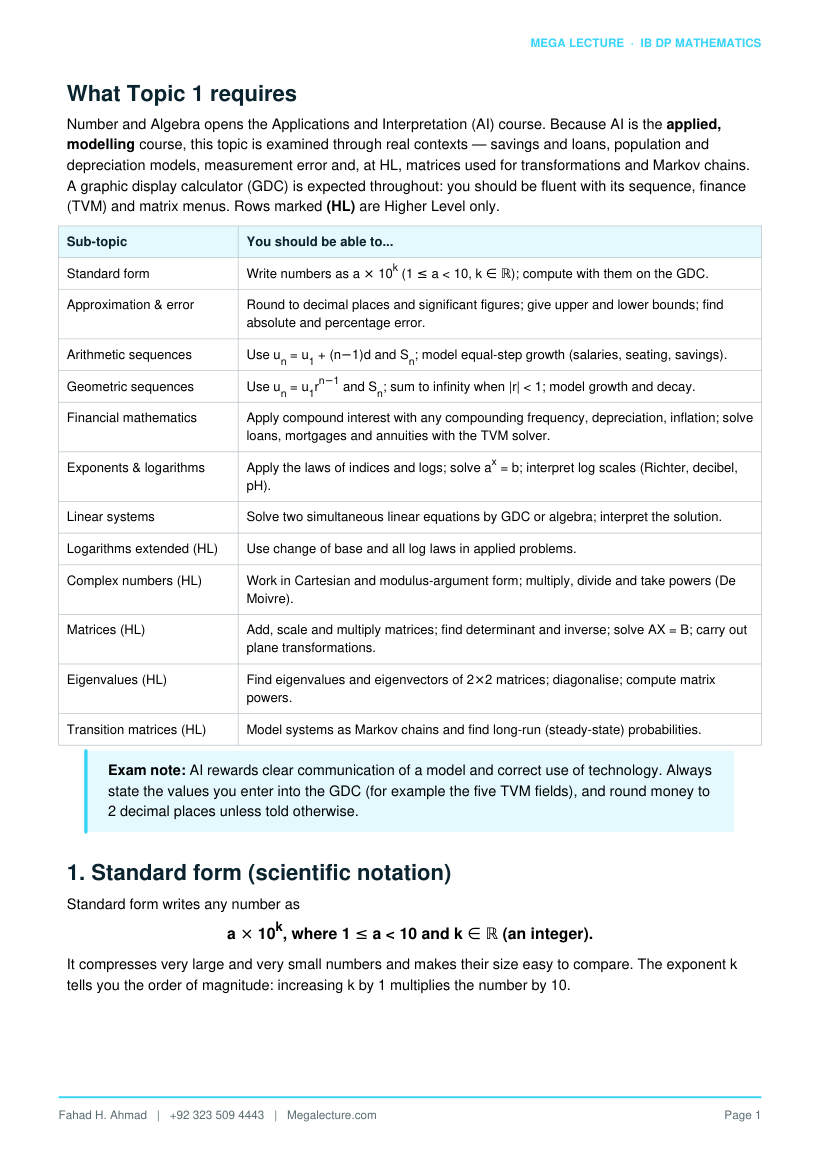
What Topic 1 requires

Number and Algebra opens the Applications and Interpretation (AI) course. Because AI is the applied, modelling course, this topic is examined through real contexts — savings and loans, population and depreciation models, measurement error and, at HL, matrices used for transformations and Markov chains. A graphic display calculator (GDC) is expected throughout: you should be fluent with its sequence, finance (TVM) and matrix menus. Rows marked (HL) are Higher Level only.

Sub-topic You should be able to...

Standard form Write numbers as a × 10k (1 ≤ a < 10, k ∈ ℝ); compute with them on the GDC.

Approximation & error Round to decimal places and significant figures; give upper and lower bounds; find absolute and percentage error.

Arithmetic sequences Use un = u1 + (n−1)d and Sn; model equal-step growth (salaries, seating, savings).

Geometric sequences Use un = u1rn−1 and Sn; sum to infinity when |r| < 1; model growth and decay.

Financial mathematics Apply compound interest with any compounding frequency, depreciation, inflation; solve loans, mortgages and annuities with the TVM solver.

Exponents & logarithms Apply the laws of indices and logs; solve ax = b; interpret log scales (Richter, decibel, pH).

Linear systems Solve two simultaneous linear equations by GDC or algebra; interpret the solution.

Logarithms extended (HL) Use change of base and all log laws in applied problems.

Complex numbers (HL) Work in Cartesian and modulus-argument form; multiply, divide and take powers (De Moivre).

Matrices (HL) Add, scale and multiply matrices; find determinant and inverse; solve AX = B; carry out plane transformations.

Eigenvalues (HL) Find eigenvalues and eigenvectors of 2×2 matrices; diagonalise; compute matrix powers.

Transition matrices (HL) Model systems as Markov chains and find long-run (steady-state) probabilities.

Exam note: AI rewards clear communication of a model and correct use of technology. Always state the values you enter into the GDC (for example the five TVM fields), and round money to 2 decimal places unless told otherwise.

1. Standard form (scientific notation)

Standard form writes any number as a × 10k, where 1 ≤ a < 10 and k ∈ ℝ (an integer).

It compresses very large and very small numbers and makes their size easy to compare. The exponent k tells you the order of magnitude: increasing k by 1 multiplies the number by 10.

Ordinary number Standard form Reading

48 000 000 4.8 × 107 move the point 7 places left

0.000 062 6.2 × 10−5 move the point 5 places right

9.1 × 10−31 kg mass of an electron very small → negative k

Operating with standard form

• Multiply / divide: multiply (or divide) the values a, and add (or subtract) the exponents, then re-standardise so that 1 ≤ a < 10.
• Add / subtract: first rewrite both numbers with the same power of 10, then add the values.
• On the GDC: use the EE or ×10x key rather than typing "10^"; the calculator keeps full precision and displays the answer in scientific notation.

Worked example 1 — standard form

Evaluate (6.0 × 108) × (5.0 × 10−3), giving the answer in standard form.

Values: 6.0 × 5.0 = 30. Exponents: 8 + (−3) = 5. So the raw answer is 30 × 105.

Re-standardise: 30 = 3.0 × 101, hence the answer is 3.0 × 106.

2. Approximation, bounds and error

Every measurement and every rounded value carries uncertainty. AI expects you to round correctly, state bounds, and quantify how far an approximation lies from the true value.

Rounding

• Decimal places (d.p.): count digits after the point. 3.14159 to 2 d.p. is 3.14.
• Significant figures (s.f.): count from the first non-zero digit. 0.004070 to 3 s.f. is 0.00407; 48 250 to 2 s.f. is 48 000.

Upper and lower bounds

A value rounded to a given accuracy could have come from a range of true values. If a length is 84 cm to the nearest cm, the true length x satisfies

83.5 ≤ x < 84.5.

The bound is half of the rounding unit either side. Carry bounds through calculations to find the largest and smallest possible results.

Absolute and percentage error

If vA is the approximate (or measured) value and vE is the exact value, then absolute error = |vA − vE| percentage error = ( |vA − vE| / |vE| ) × 100%

Worked example 2 — percentage error

A student measures a metal rod as 2.5 m. Its true length is 2.54 m. Find the absolute error and the percentage error.

Absolute error = |2.5 − 2.54| = 0.04 m.

Percentage error = (0.04 / 2.54) × 100% = 1.5748... % ≈ 1.57%.

Note the exact value vE goes in the denominator, not the measured value — a common slip.

Common pitfall: Percentage error always divides by the exact value |vE|. Dividing by the approximation gives a slightly wrong figure and loses marks.

Working with bounds

When rounded quantities are combined, propagate the bounds: use the two extreme values that could have produced each rounded figure to get the largest and smallest possible result.

Worked example 2b - bounds in a calculation

A rectangular plot is measured as 12 m by 8 m, each to the nearest metre. Find the upper and lower bounds for its area.

Length: 11.5 ≤ L < 12.5. Width: 7.5 ≤ Wd < 8.5.

Lower bound area = 11.5 × 7.5 = 86.25 m2.

Upper bound area = 12.5 × 8.5 = 106.25 m2.

So the true area lies in 86.25 ≤ A < 106.25 m2 - a wide range from small measurement uncertainty.

3. Arithmetic sequences and series

An arithmetic sequence changes by a constant common difference d each term: it models any quantity that grows or shrinks by equal steps, such as a fixed annual pay rise or a simple-interest savings plan.

un = u1 + (n − 1)d Sn = (n/2)(2u1 + (n − 1)d) = (n/2)(u1 + un)

Here un is the n-th term, u1 the first term, and Sn the sum of the first n terms. The two forms of Sn are equivalent; use whichever fits the information given.

Worked example 3 — a real-life arithmetic model

A theatre has 24 seats in the front row, and each row behind has 2 more seats than the one in front. There are 30 rows. How many seats are in the back row, and how many seats in total?

Arithmetic with u1 = 24, d = 2, n = 30.

Back row: u30 = 24 + (30 − 1)(2) = 24 + 58 = 82 seats.

Total: S30 = (30/2)(24 + 82) = 15 × 106 = 1590 seats.

Figure 2. Arithmetic versus geometric growth over eight terms. The arithmetic sequence (u1 = 2, d = 3) rises by equal steps;

the geometric sequence (u1 = 2, r = 1.7) multiplies each term and overtakes it at the fifth term.

4. Geometric sequences and series

A geometric sequence multiplies by a constant common ratio r each term. It models percentage growth and decay — compound interest, population change, radioactive decay, depreciation — because a fixed percentage change is a fixed multiplier.

un = u1 rn−1 Sn = u1(rn − 1)/(r − 1) = u1(1 − rn)/(1 − r), r ≠ 1

Sum to infinity

If |r| < 1 the terms shrink towards zero and the series converges to a finite total:

S∞ = u1 / (1 − r), valid only for |r| < 1.

Figure 4. Partial sums Sn of the convergent geometric series (a = 12, r = 0.5) climb towards the sum to infinity S∞ = a/(1 − r)

= 24 (dashed line).

Worked example 4 — geometric growth and a limit

A geometric sequence has u1 = 3 and r = 2. (a) Find u10 and S10. (b) A different sequence has u1 = 12 and r = 0.5; find its sum to infinity.

• u10 = 3 × 29 = 3 × 512 = 1536.

S10 = 3(210 − 1)/(2 − 1) = 3(1024 − 1) = 3 × 1023 = 3069.

• |r| = 0.5 < 1, so S∞ = 12 / (1 − 0.5) = 12 / 0.5 = 24.

Worked example 4b - modelling decay with a geometric sequence

A patient is given 80 mg of a drug. Each hour the body removes 25% of the drug present, so 75% remains. (a) How much remains after 5 hours? (b) After how many whole hours does the amount first fall below 10 mg?

Geometric decay with u1 = 80 (start) and r = 0.75; amount after n hours = 80(0.75)n.

• 80(0.75)5 = 80 × 0.23730 = 18.98 mg.
• Solve 80(0.75)n < 10 ⇒ (0.75)n < 0.125 ⇒ n > log 0.125 / log 0.75 = 7.23, so first below 10 mg after 8 hours.

Common pitfall: The sum to infinity exists only when |r| < 1. If |r| ≥ 1 the terms do not shrink and the series has no finite sum — writing S∞ is then meaningless.

5. Financial mathematics

This is the signature application of AI. All of it is geometric growth in disguise, but the exam expects the finance vocabulary and confident use of the GDC finance (TVM) solver.

Compound interest

With principal (present value) PV, annual interest rate r as a decimal, compounded n times per year for t years, the future value is

FV = PV(1 + r/n)nt

The compounding frequency n matters: more frequent compounding gives a larger FV for the same quoted annual rate. Typical values are n = 1 (annually), 2 (semi-annually), 4 (quarterly), 12 (monthly), 365 (daily).

Figure 1. Compound interest on $5000 at 6% per year, A = P(1 + r/k)kn. Monthly compounding (k = 12) grows faster than annual (k = 1); after 10 years the balance is $9096.98 versus $8954.24.

Worked example 5 — compound interest, quarterly

$5000 is invested at a nominal annual rate of 6%, compounded quarterly, for 5 years. Find the future value and the interest earned.

PV = 5000, r = 0.06, n = 4, t = 5, so nt = 20 and r/n = 0.015.

FV = 5000(1 + 0.015)20 = 5000(1.015)20 = 5000 × 1.346855 = $6734.28.

Interest earned = 6734.28 − 5000 = $1734.28.

How compounding frequency changes the return

For a fixed nominal rate, compounding more often gives a larger future value. The table shows $1000 after one year at a nominal 12% for different frequencies, and the resulting effective annual rate (the single annual rate that would give the same growth).

Compounding n FV of $1000 after 1 year Effective annual rate

Annually $1120.00 12.00%

Semi-annually $1123.60 12.36%

Quarterly $1125.51 12.55%

Monthly $1126.83 12.68%

Compounding n FV of $1000 after 1 year Effective annual rate

Daily $1127.47 12.75%

The gains shrink as n grows: there is a ceiling (continuous compounding). This is why lenders quote an effective, not just nominal, rate - it lets consumers compare products fairly.

Depreciation, inflation, real value

• Depreciation: an asset losing p% of its value each year has value PV(1 − p/100)t after t years — geometric decay with r = 1 − p/100.
• Inflation: prices rising at i% per year multiply by (1 + i/100)t. What costs $100 today costs more later.
• Real vs nominal: the nominal value ignores inflation; the real value adjusts for it, showing purchasing power. An investment can grow in nominal terms yet lose real value if inflation outpaces the interest rate.

Figure 3. Exponential depreciation V = V0(1 − d)n of an $18000 car losing 15% of its value each year. After 5 years the car is worth $7986.70 (marked in red).

Worked example 5b - real versus nominal value

$10 000 is invested and grows at 5% per year for 6 years. Over the same period prices rise at 3% per year. Find the nominal value and the real (inflation-adjusted) value after 6 years.

Nominal value = 10000(1.05)6 = $13 400.96.

Real value = 13 400.96 / (1.03)6 = 13 400.96 / 1.19405 = $11 223.09 in today's money.

The investment grows in real terms because 5% > 3%; had inflation exceeded 5%, purchasing power would have fallen despite the rising balance.

The TVM (time value of money) solver

Loans, mortgages, savings plans and annuities are all solved with the calculator's finance solver, which links five quantities. Enter four and solve for the fifth.

Field Meaning Sign convention

N total number of payment periods positive

I% nominal annual interest rate as a percent positive

PV present value (loan received / initial deposit) money received is +, paid is −

PMT the regular payment opposite sign to PV

FV future value (final balance) as appropriate

P/Y, C/Y payments per year and compounding periods per year usually equal

Amortization is the gradual repayment of a loan by equal instalments: early payments are mostly interest, later payments mostly principal. The GDC amortization table shows the interest, principal and balance for any payment.

Worked example 6 — a loan repayment (annuity) via TVM

A $10 000 loan is taken at a nominal annual rate of 6%, compounded monthly, to be repaid by equal monthly payments over 3 years. Find the monthly payment and the total interest paid.

Monthly rate i = 0.06/12 = 0.005; number of payments N = 3 × 12 = 36.

PMT = PV × i / (1 − (1 + i)−N) = 10000 × 0.005 / (1 − 1.005−36) = 50 / 0.164354 = $304.22 per month.

GDC: N = 36, I% = 6, PV = 10000, FV = 0, P/Y = C/Y = 12 → PMT = −304.22.

Total paid = 304.22 × 36 = 10 951.92, so interest = 10 951.92 − 10 000 = $951.92.

Worked example 6b - a regular savings plan (future value annuity)

$150 is deposited at the end of every month into an account paying a nominal 4.8% compounded monthly. Find the value of the plan after 10 years.

Monthly rate i = 0.048/12 = 0.004; number of deposits N = 10 × 12 = 120.

FV = PMT × ((1 + i)N − 1)/i = 150 × (1.004120 − 1)/0.004 = 150 × 153.632 = $23 044.79.

GDC: N = 120, I% = 4.8, PV = 0, PMT = −150, P/Y = C/Y = 12 → FV = 23 044.79. Total deposited = 150 × 120 = 18 000, so interest earned = $5044.79.

Common pitfall: Match the period to the compounding. For monthly compounding, N counts months and the periodic rate is the annual rate divided by 12 — never put years into N when payments are monthly.

6. Exponents and logarithms

Exponents and logarithms are inverse operations: logab is the power to which a must be raised to give b. They let you solve for an unknown exponent — for instance the time for an investment to reach a target, or the order of magnitude on a log scale.

Laws of exponents Laws of logarithms am × an = am+n log(xy) = log x + log y am ÷ an = am−n log(x/y) = log x − log y

(am)n = amn log(xn) = n log x a0 = 1, a−n = 1/an logaa = 1, loga1 = 0

Solving ax = b

Take logs of both sides and use the power law:

ax = b ⇒ x log a = log b ⇒ x = log b / log a

Worked example 7 — solving with logarithms

Solve 5 × 2x = 300, giving x to 3 significant figures.

Divide by 5: 2x = 60.

Take logs: x = log 60 / log 2 = 1.77815 / 0.30103 = 5.9069... ≈ 5.91.

Check: 25.91 ≈ 60.0, and 5 × 60 = 300. ⇒ correct.

Logarithmic scales as applications

A log scale compresses a huge range of values so each step of 1 unit multiplies the underlying quantity by a fixed factor.

Scale Measures Key idea

Richter (M) earthquake amplitude each unit = ×10 amplitude (about ×32 energy)

Decibel (dB) sound intensity level L = 10 log(I/I0); +10 dB = ×10 intensity pH acidity, pH = −log[H+] each unit = ×10 hydrogen-ion concentration

Worked example 7b - a logarithmic scale in context

A solution has hydrogen-ion concentration [H+] = 3.2 × 10−5 mol dm−3. Find its pH, and state how the concentration changes if the pH rises by 2.

pH = −log[H+] = −log(3.2 × 10−5) = −(log 3.2 − 5) = −(0.505 − 5) = 4.49.

Each pH unit is a factor of 10 in [H+], so a rise of 2 in pH means [H+] falls by a factor of 102 = 100 (the solution becomes less acidic).

7. Systems of linear equations

Two linear equations in two unknowns represent two straight lines. Solving them finds where the lines meet — the pair (x, y) satisfying both. AI problems phrase this as balancing two conditions, for example two pricing plans that give the same cost.

• One solution: lines cross once (different gradients).
• No solution: parallel, distinct lines (same gradient, different intercept).
• Infinitely many: the two equations describe the same line.

Solve by elimination or substitution, or enter the system into the GDC's simultaneous-equation solver. For example, 2x + 3y = 12 and x − y = 1 give x = 3, y = 2 (check: 6 + 6 = 12 and 3 − 2 = 1). At HL the same idea extends to matrices (Section 10).

Technology tip: The GDC linear-system solver gives exact intersections instantly and flags when a system has no unique solution — use it to check hand-algebra under exam time pressure.

8. Logarithms extended (HL)

At HL the log laws are used more freely, and the change-of-base rule lets you evaluate a logarithm to any base on a calculator that only offers base 10 and base e:

logab = logcb / logca (any convenient base c)

Combined with the product, quotient and power laws, this condenses or expands complicated expressions and solves exponential-model equations that mix bases. A frequent application is finding the time in a growth or decay model N = N0at: rearranging gives t = log(N/N0) / log a.

Worked example 8 (HL) — condensing and solving

Write 2 log x + log 3 − log 12 as a single logarithm, then solve 2 log x + log 3 = log 12 for x > 0.

2 log x + log 3 − log 12 = log x2 + log 3 − log 12 = log(3x2/12) = log(x2/4).

Setting log(x2/4) = 0 gives x2/4 = 1, so x2 = 4 and, since x > 0, x = 2.

9. Complex numbers (HL)

A complex number extends the reals by the imaginary unit i, where i2 = −1. It is written in Cartesian form z = a + bi, with real part a and imaginary part b. Complex numbers ∈ ℂ let us handle quantities with both size and phase.

Modulus-argument (polar) form

Plotting z on an Argand diagram, its distance from the origin is the modulus and its angle from the positive real axis is the argument:

|z| = r = √(a2 + b2) θ = arg z = arctan(b/a) z = r(cos θ + i sin θ)

Operations

• Add / subtract: in Cartesian form, combine real and imaginary parts separately.
• Multiply / divide: easiest in polar form — multiply the moduli and add the arguments (divide the moduli and subtract the arguments).
• Powers (De Moivre): zn = rn(cos nθ + i sin nθ).

Worked example 9 (HL) — polar form and De Moivre

For z = 1 + i, find |z| and arg z, then use De Moivre to evaluate z8.

|z| = √(12 + 12) = √2; arg z = arctan(1/1) = π/4 (45°).

z8 = (√2)8(cos(8 × 45°) + i sin(8 × 45°)) = 16(cos 360° + i sin 360°) = 16(1 + 0i) = 16.

Where it is used

In modelling, the modulus-argument form captures an amplitude and a phase angle at once. This is exactly how alternating-current (AC) circuits and oscillations are analysed: a voltage or current is represented by a phasor — a complex number whose modulus is the amplitude and whose argument is the phase — so that combining signals becomes complex addition. The treatment in AI is conceptual: recognise why complex numbers are the natural language here.

10. Matrices (HL)

A matrix is a rectangular array of numbers. Its order is rows × columns; a 2×3 matrix has 2 rows and 3 columns. Matrices store and transform data efficiently and underpin the transition-matrix and transformation models later in this topic.

Notation used below: a 2×2 matrix with rows (a b) and (c d) is written ( a b ; c d ), the semicolon separating the two rows.

Basic operations

• Addition / subtraction: only for matrices of the same order; add corresponding entries.
• Scalar multiple: multiply every entry by the scalar.
• Multiplication: A (×) B is defined only when the columns of A equal the rows of B; entry (i, j) is the row-i of A dotted with column-j of B. Matrix multiplication is not commutative: in general AB ≠ BA.
• Identity I ( 1 0 ; 0 1 ) leaves any matrix unchanged (AI = IA = A); the zero matrix has every entry 0.

Determinant and inverse of a 2×2 matrix

For A = ( a b ; c d ):

det A = ad − bc A−1 = (1/det A) ( d −b ; −c a ), provided det A ≠ 0.

If det A = 0 the matrix is singular and has no inverse. For 3×3 matrices, find the determinant and inverse with the GDC.

Solving systems with matrices

A linear system can be written AX = B, where A holds the coefficients, X the unknowns and B the constants. If A is invertible, X = A−1B.

Worked example 10 (HL) — multiply, invert, solve

Let A = ( 1 2 ; 3 4 ) and B = ( 2 0 ; 1 3 ). (a) Find AB. (b) Find A−1. (c) Solve x + 2y = 5, 3x + 4y = 6.

• AB = ( 1·2+2·1 1·0+2·3 ; 3·2+4·1 3·0+4·3 ) = ( 4 6 ; 10 12 ).
• det A = (1)(4) − (2)(3) = −2, so A−1 = (−1/2)( 4 −2 ; −3 1 ) = ( −2 1 ; 1.5 −0.5 ).
• AX = B with B = ( 5 ; 6 ). X = A−1B = ( −2·5 + 1·6 ; 1.5·5 + (−0.5)·6 ) = ( −4 ; 4.5 ), so x = −4, y = 4.5.

Check: −4 + 2(4.5) = 5 ⇒ and 3(−4) + 4(4.5) = −12 + 18 = 6 ⇒.

Matrix transformations of the plane

Multiplying position vectors by a 2×2 matrix transforms the whole plane. The area scale factor of the transformation is |det| — the factor by which every area is multiplied.

Transformation Matrix det

Rotation by θ about O ( cos θ −sin θ ; sin θ cos θ )

Reflection in the x-axis ( 1 0 ; 0 −1 ) −1

Reflection in the y-axis ( −1 0 ; 0 1 ) −1

Enlargement, scale factor k (k0;0k) k2

Figure 5. A 90° rotation, matrix ( 0 −1 ; 1 0 ), maps the triangle (1, 0), (3, 0), (1, 2) to (0, 1), (0, 3), (−2, 1). The determinant is

1, so area is preserved.

Common pitfall: Order matters. To apply transformation P then Q to a vector, compute Q(Pv) = (QP)v — the second transformation's matrix goes on the left. And if det A = 0 there is no inverse, so AX = B cannot be solved this way.

11. Eigenvalues, eigenvectors and matrix powers (HL)

For a square matrix M, a non-zero vector v is an eigenvector with eigenvalue λ if multiplying by M only stretches v (it keeps its direction):

Mv = λv found from det(M − λI) = 0.

For a 2×2 matrix the equation det(M − λI) = 0 is a quadratic in λ (the characteristic equation). Solve it for the eigenvalues, then substitute each back to find the matching eigenvectors.

Diagonalisation and powers

If M has eigenvalues λ1, λ2 with eigenvectors forming the columns of P, then M = PDP−1, where D = ( λ1 0 ; 0 λ2 ). This makes high powers easy, because

Mn = P Dn P−1, and Dn = ( λ1 n 0 ; 0 λ2 n ).

Raising a diagonal matrix to a power just raises each diagonal entry to that power — far cheaper than multiplying M by itself n times, and the key to long-run behaviour of transition matrices.

Worked example 11 (HL) — eigenvalues and eigenvectors

Find the eigenvalues and eigenvectors of M = ( 2 1 ; 1 2 ).

det(M − λI) = (2 − λ)2 − 1 = λ2 − 4λ + 3 = 0, so (λ − 1)(λ − 3) = 0 and λ = 1 or 3.

λ = 3: (2 − 3)x + y = 0 ⇒ y = x, eigenvector ( 1 ; 1 ).

λ = 1: (2 − 1)x + y = 0 ⇒ y = −x, eigenvector ( 1 ; −1 ).

Worked example 11b (HL) - a matrix power by diagonalisation

Using M = ( 2 1 ; 1 2 ) from Worked example 11 (eigenvalues λ = 3, 1), find M4.

Take P = ( 1 1 ; 1 −1 ) (eigenvectors as columns) and D = ( 3 0 ; 0 1 ). Then M4 = P D4 P−1 with D4 = ( 81 0 ; 0 1 ).

det P = −2, so P−1 = (−1/2)( −1 −1 ; −1 1 ) = ( 0.5 0.5 ; 0.5 −0.5 ).

M4 = ( 1 1 ; 1 −1 )( 81 0 ; 0 1 )( 0.5 0.5 ; 0.5 −0.5 ) = ( 41 40 ; 40 41 ).

Check directly: M2 = ( 5 4 ; 4 5 ), and (M2)2 = ( 41 40 ; 40 41 ) ⇒ confirmed.

12. Transition (Markov) matrices and steady state (HL)

A transition matrix T models a system that moves between a fixed set of states in steps, where the next state depends only on the current one (a Markov chain). Each column lists the probabilities of moving from one state, so every column sums to 1. If sk is the state (probability) vector after k steps, then sk+1 = T sk, and after n steps sn = Tn s0.

Long-run (steady state)

For many chains the state vector settles to a steady state s that no longer changes: T s = s. This s is an eigenvector of T with eigenvalue 1, scaled so its entries sum to 1. Solve the linear equations T s = s together with the constraint that the probabilities add to 1.

Worked example 12 (HL) — steady-state probabilities

Each week commuters switch between car and bus. Of car users, 80% keep the car and 20% switch to bus; of bus users, 30% switch to car and 70% keep the bus. Find the long-run share using each mode.

With states (car, bus), the transition matrix (columns = current mode) is T = ( 0.8 0.3 ; 0.2 0.7 ).

Steady state s = ( c ; b ) with T s = s: 0.8c + 0.3b = c ⇒ 0.3b = 0.2c ⇒ c = 1.5b.

Using c + b = 1: 1.5b + b = 1 ⇒ 2.5b = 1 ⇒ b = 0.4, c = 0.6.

Long run: 60% travel by car and 40% by bus. Check: 0.8(0.6) + 0.3(0.4) = 0.48 + 0.12 = 0.6 ⇒.

Figure 6. The commuter Markov chain T = ( 0.8 0.3 ; 0.2 0.7 ) started from all-car. The state probabilities converge to the steady state ( 0.6 ; 0.4 ) (dashed), whatever the starting split.

Interpretation: The steady state is independent of the starting split — whatever the initial shares, repeated application of T drives the system to the same long-run distribution.

13. Common pitfalls checklist

• Dividing by the measured value instead of the exact value when computing percentage error.
• Forgetting to re-standardise (1 ≤ a < 10) after multiplying numbers in standard form.
• Using the sum to infinity when |r| ≥ 1 — it only exists for |r| < 1.
• Mismatching the compounding period with N in the TVM solver (years vs months).
• Sign errors in the TVM solver: money paid out and money received must have opposite signs.
• Assuming AB = BA for matrices — multiplication order changes the result (HL).
• Trying to invert a matrix with det = 0 — no inverse exists, so AX = B has no unique solution (HL).
• Writing transition-matrix columns that do not sum to 1 (HL).

14. Quick-reference formulae

Idea Formula

Standard form a × 10k, 1 ≤ a < 10, k ∈ ℝ

Percentage error ( |vA − vE| / |vE| ) × 100%

Arithmetic term / sum un = u1 + (n−1)d; Sn = (n/2)(2u1 + (n−1)d)

Geometric term / sum un = u1rn−1; Sn = u1(rn−1)/(r−1)

Sum to infinity (|r|<1) S∞ = u1/(1−r)

Compound interest FV = PV(1 + r/n)nt

Depreciation value = PV(1 − p/100)t

Solve exponential ax = b ⇒ x = log b / log a

Change of base (HL) logab = logcb / logca

Complex modulus/arg (HL) |z| = √(a2+b2); zn = rn(cos nθ + i sin nθ)

2×2 inverse (HL) A−1 = (1/(ad−bc))( d −b ; −c a )

Area scale factor (HL) |det A|

Eigenvalues (HL) det(M − λI) = 0; Mn = PDnP−1

Steady state (HL) T s = s, entries of s sum to 1

15. Practice questions

Attempt all ten without a solutions sheet; use your GDC as you would in the exam. Full worked answers follow. Questions marked (HL) are Higher Level.

• Evaluate (3.2 × 105)(4.0 × 10−2) in standard form.
• A value of 1/3 is approximated as 0.33. Find the percentage error, to 2 s.f.
• An arithmetic sequence has u1 = 5 and d = 3. Find S20.
• A geometric sequence has u1 = 8 and r = 1/4. Find its sum to infinity.
• $2000 is invested at 3.5% per year compounded monthly for 4 years. Find the future value.
• A car worth $18 000 depreciates by 15% per year. Find its value after 5 years.
• Solve 3x = 50, giving x to 3 s.f.
• (HL) For z = 3 + 4i, find |z| and arg z (in degrees, to 1 d.p.).
• (HL) For A = ( 3 1 ; 2 4 ), find det A and A−1.
• (HL) A Markov chain has T = ( 0.9 0.5 ; 0.1 0.5 ). Find the steady-state vector.
• A town of 5000 people grows by 4% each year. Find the population after 8 years, and the number of whole years for it to first exceed 8000.
• (HL) Given z1 = 2(cos 30° + i sin 30°) and z2 = 3(cos 45° + i sin 45°), find z1z2 in polar form.

Worked answers

• Values: 3.2 × 4.0 = 12.8; exponents 5 + (−2) = 3, giving 12.8 × 103. Re-standardise: 1.28 × 104.
• vE = 0.33333..., vA = 0.33. Error = |0.33 − 0.33333| = 0.003333. Percentage = (0.003333 / 0.33333) × 100% ≈ 1.0%.
• S20 = (20/2)(2·5 + (20−1)·3) = 10(10 + 57) = 10 × 67 = 670.
• |r| = 0.25 < 1, so S∞ = 8/(1 − 0.25) = 8/0.75 = 32/3 ≈ 10.67.
• FV = 2000(1 + 0.035/12)48 = 2000(1.0029167)48 = 2000 × 1.1500380 ≈ $2300.08.
• Value = 18000(1 − 0.15)5 = 18000(0.85)5 = 18000 × 0.443705 ≈ $7986.70.
• x = log 50 / log 3 = 1.69897 / 0.47712 = 3.5609... ≈ 3.56.
• (HL) |z| = √(32 + 42) = √25 = 5; arg z = arctan(4/3) = 53.1°. So z = 5(cos 53.1° + i sin 53.1°).
• (HL) det A = (3)(4) − (1)(2) = 10; A−1 = (1/10)( 4 −1 ; −2 3 ) = ( 0.4 −0.1 ; −0.2 0.3 ).
• (HL) T s = s with s = ( p ; q ): 0.9p + 0.5q = p ⇒ 0.5q = 0.1p ⇒ p = 5q. With p + q = 1: 6q = 1, so q = 1/6 and p = 5/6. Steady state ( 5/6 ; 1/6 ) ≈ (0.833 ; 0.167).
• After 8 years: 5000(1.04)8 = 5000 × 1.368569 ≈ 6843 people. Exceeds 8000 when 1.04n > 1.6, i.e. n > log 1.6 / log 1.04 = 11.98, so after 12 years.
• (HL) Multiply moduli and add arguments: 2 × 3 = 6 and 30° + 45° = 75°, so z1z2 = 6(cos 75° + i sin 75°).