Topic 5: Calculus

IB DP MATHEMATICS Applications and Interpretation (AI) Topic 5 Calculus

Revision Notes · Standard and Higher Level Fahad H. Ahmad

+92 323 509 4443 | Megalecture.com

Original notes prepared for the IB Diploma Programme Mathematics AI course (first assessment 2021)

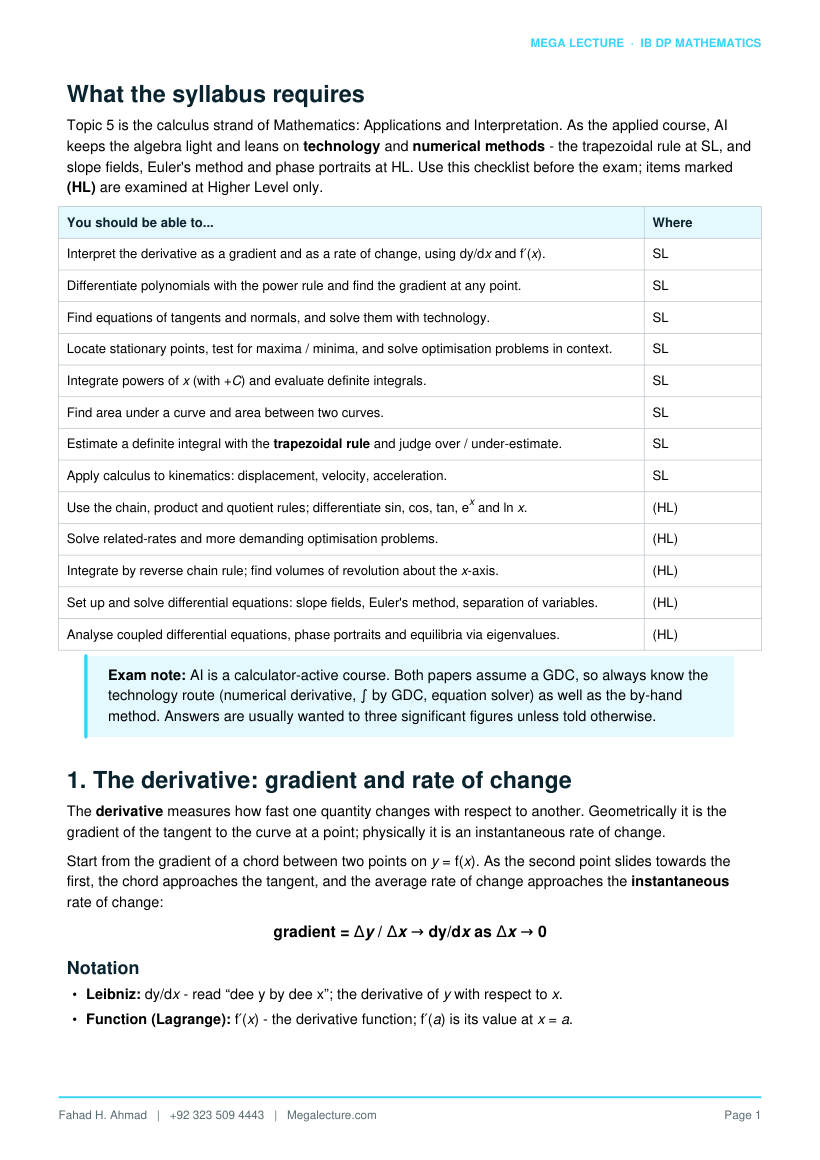
What the syllabus requires

Topic 5 is the calculus strand of Mathematics: Applications and Interpretation. As the applied course, AI keeps the algebra light and leans on technology and numerical methods - the trapezoidal rule at SL, and slope fields, Euler's method and phase portraits at HL. Use this checklist before the exam; items marked (HL) are examined at Higher Level only.

You should be able to... Where

Interpret the derivative as a gradient and as a rate of change, using dy/dx and f′(x). SL

Differentiate polynomials with the power rule and find the gradient at any point. SL

Find equations of tangents and normals, and solve them with technology. SL

Locate stationary points, test for maxima / minima, and solve optimisation problems in context. SL

Integrate powers of x (with +C) and evaluate definite integrals. SL

Find area under a curve and area between two curves. SL

Estimate a definite integral with the trapezoidal rule and judge over / under-estimate. SL

Apply calculus to kinematics: displacement, velocity, acceleration. SL

Use the chain, product and quotient rules; differentiate sin, cos, tan, ex and ln x. (HL)

Solve related-rates and more demanding optimisation problems. (HL)

Integrate by reverse chain rule; find volumes of revolution about the x-axis. (HL)

Set up and solve differential equations: slope fields, Euler's method, separation of variables. (HL)

Analyse coupled differential equations, phase portraits and equilibria via eigenvalues. (HL)

Exam note: AI is a calculator-active course. Both papers assume a GDC, so always know the technology route (numerical derivative, ∫ by GDC, equation solver) as well as the by-hand method. Answers are usually wanted to three significant figures unless told otherwise.

1. The derivative: gradient and rate of change

The derivative measures how fast one quantity changes with respect to another. Geometrically it is the gradient of the tangent to the curve at a point; physically it is an instantaneous rate of change.

Start from the gradient of a chord between two points on y = f(x). As the second point slides towards the first, the chord approaches the tangent, and the average rate of change approaches the instantaneous rate of change:

gradient = Δy / Δx → dy/dx as Δx → 0

Notation

• Leibniz: dy/dx - read “dee y by dee x”; the derivative of y with respect to x.
• Function (Lagrange): f′(x) - the derivative function; f′(a) is its value at x = a.
• A positive derivative means y is increasing; a negative derivative means it is decreasing; zero means a stationary (flat) point.
• Units matter. If V is in litres and t in seconds, then dV/dt is in litres per second - a rate.

Interpreting in context: In an applied question, always state the meaning of a derivative with units. If C(x) is cost in dollars for x items, then C′(x) is the marginal cost in dollars per extra item.

2. Differentiating polynomials: the power rule

For AI, differentiation by hand is limited to powers of x. The single rule you need is the power rule:

if y = xn then dy/dx = n xn−1

Combine it with two facts: a constant multiple stays attached (d/dx of k f(x) is k f′(x)), and you differentiate a sum term by term. The derivative of a constant is 0.

Function Derivative Comment y = x5 5x4 power rule y = 7x3 21x2 constant multiple y = 4x since x1 → 1 y = 9 constant y = x2 − 6x + 1 2x − 6 term by term y = 3/x = 3x−1 −3x−2 = −3/x2 negative index (HL-style rewrite)

Method: Before differentiating, rewrite roots and fractions as powers: √x = x1/2 and 1/x2 = x−2. Bring the index down, then subtract one from the index.

3. Gradient at a point; tangents and normals

The gradient of the curve at x = a is f′(a). From it you build two straight lines through the point (a, f(a)):

• The tangent touches the curve and has gradient m = f′(a).
• The normal is perpendicular to the tangent, so its gradient is −1/m (provided m ≠ 0).

Both lines use y − y1 = m(x − x1).

Worked example 1 - tangent and normal

Find the equations of the tangent and normal to y = x2 − 4x + 5 at the point where x = 3.

Point: y(3) = 9 − 12 + 5 = 2, so the point is (3, 2).

Gradient: dy/dx = 2x − 4, so f′(3) = 6 − 4 = 2.

Tangent: y − 2 = 2(x − 3) → y = 2x − 4.

Normal gradient = −1/2, so y − 2 = −½(x − 3) → y = −0.5x + 3.5.

Check: at x = 3 both give y = 2, and 2 × (−0.5) = −1, confirming they are perpendicular.

Figure 1. The derivative as the gradient of a tangent. The red line is drawn with the exact slope f′(3) = 2 and touches y = x2 −

4x + 5 at (3, 2), matching Worked example 1.

Technology: On the GDC, the numerical derivative gives f′(3) directly, and “tangent line” on a graphing app writes the equation for you - a fast check under exam pressure.

4. Increasing / decreasing, stationary points, optimisation

The sign of the first derivative tells you where a function rises or falls, and the derivative being zero locates the turning points that optimisation questions are built on.

Condition Meaning f′(x) > 0 on an interval f is increasing there f′(x) < 0 on an interval f is decreasing there f′(x) = 0 at x = a stationary point (local max, local min, or inflexion)

Classifying a stationary point

• First-derivative test: if f′ changes + → − it is a local maximum; − → + a local minimum.
• Second-derivative test: if f′′(a) < 0 it is a maximum; if f′′(a) > 0 it is a minimum.

For an optimisation problem: write the quantity to be optimised as a function of one variable (use a constraint to eliminate the other), differentiate, set the derivative to zero, solve, and confirm it is the maximum or minimum you want. Always check the answer is physically sensible and lies inside the domain.

Worked example 2 - optimisation (open box)

An open-top box is made from a 24 cm × 24 cm square of card by cutting a square of side x from each corner and folding up the sides. Find the value of x that maximises the volume.

Volume: V = x(24 − 2x)2 = 4x3 − 96x2 + 576x, with 0 < x < 12.

dV/dx = 12x2 − 192x + 576 = 12(x − 4)(x − 12).

Stationary points at x = 4 and x = 12. Only x = 4 is inside the domain (x = 12 gives zero volume).

Second derivative: d2V/dx2 = 24x − 192; at x = 4 this is −96 < 0, so a maximum.

Maximum volume: V = 4(24 − 8)2 = 4 × 256 = 1024 cm3 at x = 4 cm.

Figure 2. Optimisation of the open-top box. The volume V(x) = x(24 − 2x)2 has a horizontal tangent where V′(x) = 0 at x = 4 cm, giving the maximum V = 1024 cm3 (Worked example 2); the turning point is marked.

5. Integration as anti-differentiation

Integration reverses differentiation. Because the derivative of any constant is zero, an indefinite integral always carries an arbitrary constant of integration +C:

∫ xn dx = xn+1 / (n+1) + C, n ≠ −1

Integrate term by term, exactly reversing the power rule: add one to the index, then divide by the new index. A definite integral has limits and gives a number - no +C is needed because it cancels:

∫a b f(x) dx = F(b) − F(a), where F′(x) = f(x)

Worked example 3 - definite integral

Evaluate ∫1

4 (3x2 + 2) dx.

Antiderivative: F(x) = x3 + 2x.

F(4) = 64 + 8 = 72; F(1) = 1 + 2 = 3.

Value = 72 − 3 = 69.

Do not forget +C: Every indefinite integral needs +C. If a boundary condition is given (for example a point on the curve, or an initial displacement), substitute it to find C - this is how you recover a specific function from its derivative.

6. Area under a curve and between curves

The definite integral ∫a b f(x) dx equals the signed area between the curve and the x-axis. Area above the axis counts positive, area below counts negative.

• For the true area of a region that dips below the axis, integrate the parts separately and add magnitudes, or integrate |f(x)|.
• For the area between two curves on [a, b], integrate (top − bottom):

Area = ∫a b [ ytop − ybottom ] dx

Worked example 4 - area between curves

Find the area enclosed between the line y = x + 2 and the parabola y = x2.

Intersections: x2 = x + 2 → x2 − x − 2 = 0 → (x − 2)(x + 1) = 0, so x = −1 and x = 2.

On this interval the line is above the parabola, so

Area = ∫−1

2 [(x + 2) − x2] dx = [ x2/2 + 2x − x3/3 ]−1 2.

At x = 2: 2 + 4 − 8/3 = 10/3. At x = −1: 0.5 − 2 + 1/3 = −7/6.

Area = 10/3 − (−7/6) = 4.5 (square units).

7. The trapezoidal rule (AI-specific)

When a function is awkward or given only as data, the trapezoidal rule estimates the area under it by slicing the interval [a, b] into n strips of equal width h = (b − a) / n and treating each strip as a trapezium:

∫a b y dx ≈ ½h [ y0 + yn + 2(y1 + y2 + … + yn−1) ]

In words: half the width, times (the two ends, plus twice every value in between). The y-values are the heights of the curve at the strip boundaries.

Over- or under-estimate?

• If the curve is concave up (bends upward, cupped like a smile) each trapezium lies above the curve, so the rule over-estimates.
• If the curve is concave down (bends downward) the trapezia lie below the curve, so the rule under-estimates.
• More strips (larger n, smaller h) gives a better estimate.

Worked example 5 - trapezoidal rule

Estimate ∫0

2 (x2 + 1) dx using the trapezoidal rule with 4 strips.

Width: h = (2 − 0)/4 = 0.5, giving x = 0, 0.5, 1, 1.5, 2.

Heights y = x2 + 1: 1, 1.25, 2, 3.25, 5.

Estimate = ½(0.5)[ 1 + 5 + 2(1.25 + 2 + 3.25) ] = 0.25[ 6 + 2(6.5) ] = 0.25(19) = 4.75.

Exact value = [x3/3 + x]0

2 = 8/3 + 2 ≈ 4.667. The estimate 4.75 is an over-estimate, as expected since y = x2 + 1 is concave up.

Figure 3. Trapezoidal rule for ∫0

2 (x2 + 1) dx with 4 strips at x = 0, 0.5, 1, 1.5, 2. The trapezia (red) sit above the shaded exact region: estimate 4.75 vs exact 14/3 ≈ 4.667, an over-estimate of +0.083 because the curve is concave up.

8. Kinematics: displacement, velocity, acceleration

Calculus links the three quantities of straight-line motion. Differentiating steps down the chain; integrating steps back up (and needs a boundary condition to fix the constant).

From Differentiate → Integrate →

Displacement s(t) velocity v = ds/dt -

Velocity v(t) acceleration a = dv/dt displacement s = ∫ v dt

Acceleration a(t) - velocity v = ∫ a dt

• Displacement over [t1, t2] = ∫t1 t2 v dt (signed).
• Distance travelled = ∫t1 t2 |v| dt; split the integral wherever v = 0 (a change of direction) and add magnitudes.
• The object is momentarily at rest when v = 0, and moving at maximum speed when a = 0.

Worked example 6 - kinematics

A particle moves in a straight line with velocity v(t) = 3t2 − 12t + 9 (m s−1) for 0 ≤ t ≤ 4 s. Find (a) when it is at rest, (b) the acceleration at t = 1, (c) the distance travelled in the first 4 s.

• v = 0: 3(t − 1)(t − 3) = 0 → t = 1 s and t = 3 s.
• a = dv/dt = 6t − 12; at t = 1: 6 − 12 = −6 m s−2.
• s = ∫ v dt = t3 − 6t2 + 9t. Values: s(0) = 0, s(1) = 4, s(3) = 0, s(4) = 4. The velocity changes sign at t = 1 and 3, so add magnitudes:

distance = |4 − 0| + |0 − 4| + |4 − 0| = 12 m, whereas the displacement is only s(4) − s(0) = 4 m.

Figure 4. Velocity−time graph v(t) = 3t2 − 12t + 9. Displacement is the signed area under the graph: +4, −4, +4 over [0, 1],

[1, 3], [3, 4], so the net displacement is 4 m while the total distance travelled is 12 m (Worked example 6).

Distance vs displacement: If asked for total distance and the velocity changes sign, you must break the interval at the roots of v(t) = 0. Integrating straight through gives displacement, not distance - a classic lost mark.

9. Further differentiation (HL)

At HL the toolkit widens to three rules and a set of standard derivatives. Let u and v be functions of x.

Rule Statement

Chain rule if y = f(u) and u = g(x), then dy/dx = (dy/du)(du/dx)

Product rule d/dx(uv) = u dv/dx + v du/dx

Rule Statement

Quotient rule d/dx(u/v) = ( v du/dx − u dv/dx ) / v2

Standard derivatives (angles in radians):

f(x) f′(x) f(x) f′(x) sin x cos x ex ex cos x −sin x ln x 1/x tan x 1 / cos2x xn n xn−1

For example, by the chain rule d/dx (3x + 1)5 = 5(3x + 1)4 × 3 = 15(3x + 1)4; and by the product rule d/dx(x2

• = 2x ex + x2 ex = x ex(x + 2).

Radians for calculus: The derivative formulae for sin and cos are only valid when x is in radians. Put your GDC in radian mode for any calculus involving trigonometric functions, or every gradient will be wrong.

10. Related rates and further optimisation (HL)

A related-rates problem links two changing quantities through an equation and asks for one rate given another. The chain rule connects them through time:

dA/dt = (dA/dr) × (dr/dt)

Method: write the relationship between the variables, differentiate both sides with respect to t, then substitute the known rate and the instantaneous values. For example, a circular oil slick with area A = πr2 has dA/dt = 2πr (dr/dt); if the radius grows at 0.5 m s−1 when r = 10 m, then dA/dt = 2π(10)(0.5) = 10π ≈ 31.4 m2 s−1.

Worked example - related rates (HL)

A spherical balloon is inflated so that its volume increases at 50 cm3 s−1. Find the rate at which the radius is increasing when r = 5 cm. (V = &frac43;πr3.)

Differentiate with respect to time: dV/dt = 4πr2 (dr/dt).

So dr/dt = (dV/dt) / (4πr2) = 50 / (4π × 25) = 1/(2π) ≈ 0.159 cm s−1.

Further optimisation: HL optimisation may combine the product or quotient rule with a constraint (surface area fixed, cost minimised). The strategy is unchanged: one variable, differentiate, set to zero, and confirm with the second derivative or a sign check.

11. Further integration and volumes of revolution (HL)

Reverse chain rule. To integrate a composite you recognise the derivative of the inner function as a factor. For instance ∫ 2x ex² dx = ex² + C, because differentiating ex² returns 2x ex². In practice AI expects most definite integrals to be evaluated by technology.

Volume of revolution about the x-axis

Rotating the region under y = f(x) from x = a to x = b a full turn about the x-axis sweeps out a solid whose volume is:

V = π ∫a b y2 dx = π ∫a

b [ f(x) ]2 dx

Each thin slice is a disc of radius y and thickness dx, with area πy2. For example, rotating y = √x for 0 ≤ x ≤ 4 gives V = π ∫0 4 x dx = π [x2/2]0 4 = 8π ≈ 25.1 cubic units.

Watch the square: In the volume formula it is y2 that is integrated, not y. Square the function first, keep the factor π outside, and give the answer as an exact multiple of π or to three significant figures.

12. Differential equations (HL)

A differential equation relates a function to its derivative. A first-order equation has the form dy/dx = f(x, y). AI treats them graphically (slope fields), numerically (Euler's method) and analytically (separation of variables).

Slope fields

At each point (x, y) the equation gives a gradient, drawn as a short line segment. The resulting field of tick-marks shows the family of solution curves without solving anything: a particular solution is the curve that follows the slopes and passes through a given initial point.

Figure 5. Slope field for dy/dx = x + y (HL). Each short segment has gradient x + y at that point; the solution curve y = 2ex − x

− 1 through (0, 1) follows the field everywhere.

Euler's method

Euler's method walks along the solution in small steps of size h, following the current gradient each time:

xn+1 = xn + h, yn+1 = yn + h × f(xn, yn)

Worked example 7 - Euler's method

Given dy/dx = x + y with y(0) = 1, use Euler's method with step h = 0.1 to estimate y(0.3).

Apply ynew = y + 0.1(x + y) three times:

n xn yn f = x+y h·f yn+1

0.0 1.000 1.000 0.100 1.100

0.1 1.100 1.200 0.120 1.220

0.2 1.220 1.420 0.142 1.362

Estimate: y(0.3) ≈ 1.362.

The exact solution is y = 2ex − x − 1, giving y(0.3) ≈ 1.400. Euler's estimate is a little low - the method under-estimates here because the solution is concave up and each step uses the gradient at the start of the interval.

Figure 6. Euler's method (HL) for dy/dx = x + y, y(0) = 1, step h = 0.1. The polygonal Euler path (red, iterates marked) lies below the true curve y = 2ex − x − 1: it gives y(0.3) ≈ 1.362 against the true 1.400, an under-estimate on this concave-up solution.

Separation of variables

If the equation can be written g(y) dy = h(x) dx, integrate both sides separately and then apply the initial condition. This gives the exact solution when it can be done.

Euler step accuracy: A smaller step h gives a more accurate result but needs more steps. Euler's method accumulates error at every step, so it systematically lags on concave-up curves and overshoots on concave-down ones. State whether your estimate is likely an over- or under-estimate.

13. Coupled differential equations and phase portraits (HL)

Two quantities that influence each other's growth (predators and prey, two competing populations, coupled tanks) are modelled by a coupled system:

dx/dt = ax + by, dy/dt = cx + dy

This is a matrix equation, linking Topic 5 to Topic 1: the vector (x, y) evolves under the 2 × 2 matrix of coefficients.

• An equilibrium (critical) point is where dx/dt = dy/dt = 0 - the system stays put there.
• A phase portrait plots trajectories in the x-y plane, showing how the state moves over time regardless of the clock.
• The eigenvalues λ of the coefficient matrix decide the behaviour near equilibrium.

Exact solutions and stability via eigenvalues

Finding eigenvalues λ and eigenvectors of the matrix gives the exact solution as a combination of eλ1t and eλ2t terms. Their signs classify the equilibrium:

Eigenvalues (real) Equilibrium type Long-term behaviour both < 0 stable node (sink) trajectories converge to equilibrium both > 0 unstable node (source) trajectories diverge away opposite signs saddle point unstable; approaches then leaves complex (non-zero real part) spiral spirals in (real part < 0) or out (> 0) complex (zero real part) centre closed orbits (cycles)

Figure 7. Phase portrait of a coupled system dx/dt = Ax (HL) with eigenvalues λ = −0.5 ± i. Because the real part is negative, the origin is a stable spiral: every trajectory spirals inward to the equilibrium.

Conceptual link: You are not expected to derive the theory - AI wants you to find eigenvalues with technology, read off the equilibrium type, and interpret the phase portrait in context (for example, whether two competing species coexist or one dies out).

14. Modelling with differential equations (HL)

The power of differential equations is that they encode a rule of change directly from a description in words.

Situation Assumption in words Equation

Population growth rate of growth proportional to size dP/dt = kP

Logistic growth growth slows as it nears a ceiling M dP/dt = kP(1 − P/M)

Newton cooling cooling rate proportional to temperature excess dT/dt = −k(T − Ts)

Mixing / dilution rate in − rate out of dissolved substance dQ/dt = (in) − (out)

Worked example 8 - Newton's law of cooling

A drink at 90°C is left in a room at 20°C. After 10 min it has cooled to 60°C. Model with dT/dt = −k(T − 20) and find the temperature after 20 min.

Separate: ∫ dT/(T − 20) = − ∫ k dt → ln(T − 20) = −kt + C.

At t = 0, T = 90: ln 70 = C, so ln((T − 20)/70) = −kt.

At t = 10, T = 60: (60 − 20)/70 = 4/7, so −10k = ln(4/7), giving k ≈ 0.0560 min−1.

At t = 20 the excess halves-of-a-power again: (T − 20)/70 = (4/7)2 = 16/49, so T − 20 = 70(16/49) ≈ 22.9.

Temperature after 20 min ≈ 42.9°C.

15. Quick reference: derivatives and integrals

Standard results (radians throughout; +C on every indefinite integral). HL-only rows are marked.

f(x) f′(x) (derivative) ∫ f(x) dx (integral) xn n xn−1 xn+1/(n+1) + C (n ≠ −1) constant k kx + C

1/x (HL) −1/x2 ln|x| + C ex (HL) ex ex + C sin x (HL) cos x −cos x + C cos x (HL) −sin x sin x + C f(x) f′(x) (derivative) ∫ f(x) dx (integral) tan x (HL) 1/cos2x (by technology)

Tool Formula

Tangent / normal y − y1 = m(x − x1); normal gradient = −1/m

Trapezoidal rule ½h[y0 + yn + 2(y1 + … + yn−1)]

Area between curves ∫a b(ytop − ybottom) dx

Volume of revolution (HL) V = π ∫a b y2 dx

Euler's method (HL) yn+1 = yn + h × f(xn, yn)

16. Common pitfalls

• Trapezoidal direction: concave-up curves are over-estimated, concave-down are under-estimated - state which and why.
• Dropping +C: an indefinite integral without +C loses a mark; use the boundary condition to find it.
• Chain rule (HL): do not forget to multiply by the derivative of the inside function - a very common slip on (3x+1)5 type terms.
• Radians for trig calculus (HL): the derivative of sin x is cos x only in radians; check GDC mode.
• Euler step size: too large a step h gives a poor estimate; error builds at every step and biases one way.
• Distance vs displacement: for total distance in kinematics, split at v = 0 and add magnitudes.
• Signed area: a region below the axis contributes a negative integral; integrate |f| for true area.
• Squaring in volumes (HL): integrate y2, not y, and keep π outside.

17. Practice questions

Attempt all ten without notes; full worked answers follow. Questions marked (HL) are Higher Level.

• Differentiate y = 4x3 − 5x2 + 7x − 2 and find the gradient at x = 2.
• Find the equation of the tangent to y = x2 − 3x at the point where x = 1.
• Find and classify the stationary points of y = x3 − 3x.
• Evaluate ∫1 3 (2x + 1) dx.
• Find the area enclosed between y = 4 − x2 and the x-axis.
• Use the trapezoidal rule with 4 strips to estimate ∫0 4 √x dx, and state whether it over- or under-estimates.
• (HL) Differentiate y = (3x + 1)5 using the chain rule.
• (HL) Differentiate y = x2 ex using the product rule.
• (HL) Find the volume when y = √x, 0 ≤ x ≤ 4, is rotated about the x-axis.
• (HL) Given dy/dx = 2x − y, y(0) = 1, use Euler's method with h = 0.2 to estimate y(0.4).

Worked answers

• dy/dx = 12x2 − 10x + 7. At x = 2: 48 − 20 + 7 = 35.
• y(1) = 1 − 3 = −2; dy/dx = 2x − 3 = −1 at x = 1. Tangent: y + 2 = −1(x − 1) → y = −x − 1.
• dy/dx = 3x2 − 3 = 0 → x = ±1. Second derivative 6x: at x = 1 (>0) a minimum (1, −2); at x = −1 (<0) a maximum (−1, 2).
• [x2 + x]1 3 = (9 + 3) − (1 + 1) = 10.
• Roots x = ±2. ∫−2 2(4 − x2) dx = [4x − x3/3]−2 2 = 16/3 − (−16/3) = 32/3 ≈ 10.7.
• h = 1; heights √x at 0,1,2,3,4: 0, 1, 1.414, 1.732, 2. Estimate = ½(1)[0 + 2 + 2(1 + 1.414 + 1.732)] = 0.5[2 + 8.293] = 5.15. Exact = (2/3)(4)3/2 ≈ 5.33, so it is an under-estimate (curve is concave down).
• (HL) dy/dx = 5(3x + 1)4 × 3 = 15(3x + 1)4.
• (HL) dy/dx = 2x ex + x2 ex = x ex(x + 2).
• (HL) V = π ∫0 4 x dx = π [x2/2]0 4 = 8π ≈ 25.1 cubic units.
• (HL) y1 = 1 + 0.2(0 − 1) = 0.800; y2 = 0.8 + 0.2(0.4 − 0.8) = 0.8 − 0.08 = 0.72. So y(0.4) ≈ 0.72.

End of Topic 5 - Calculus. Prepared as original revision material for Megalecture. For the full Mathematics AI course notes and video lessons, visit Megalecture.com.