Topic 5: Calculus

IB DP MATHEMATICS Analysis and Approaches (AA) Topic 5 Calculus

Revision Notes · Standard and Higher Level Fahad H. Ahmad

+92 323 509 4443 | Megalecture.com

Original notes prepared for the IB Diploma Programme Mathematics: Analysis and Approaches course (first assessment 2021)

What Topic 5 requires

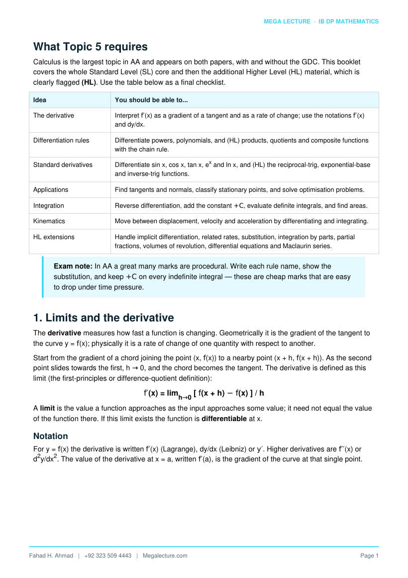
Calculus is the largest topic in AA and appears on both papers, with and without the GDC. This booklet covers the whole Standard Level (SL) core and then the additional Higher Level (HL) material, which is clearly flagged (HL). Use the table below as a final checklist.

Idea You should be able to...

The derivative Interpret f′(x) as a gradient of a tangent and as a rate of change; use the notations f′(x) and dy/dx.

Differentiation rules Differentiate powers, polynomials, and (HL) products, quotients and composite functions with the chain rule.

Standard derivatives Differentiate sin x, cos x, tan x, ex and ln x, and (HL) the reciprocal-trig, exponential-base and inverse-trig functions.

Applications Find tangents and normals, classify stationary points, and solve optimisation problems.

Integration Reverse differentiation, add the constant +C, evaluate definite integrals, and find areas.

Kinematics Move between displacement, velocity and acceleration by differentiating and integrating.

HL extensions Handle implicit differentiation, related rates, substitution, integration by parts, partial fractions, volumes of revolution, differential equations and Maclaurin series.

Exam note: In AA a great many marks are procedural. Write each rule name, show the substitution, and keep +C on every indefinite integral — these are cheap marks that are easy to drop under time pressure.

1. Limits and the derivative

The derivative measures how fast a function is changing. Geometrically it is the gradient of the tangent to the curve y = f(x); physically it is a rate of change of one quantity with respect to another.

Start from the gradient of a chord joining the point (x, f(x)) to a nearby point (x + h, f(x + h)). As the second point slides towards the first, h → 0, and the chord becomes the tangent. The derivative is defined as this limit (the first-principles or difference-quotient definition):

f′(x) = limh→0 [ f(x + h) − f(x) ] / h

A limit is the value a function approaches as the input approaches some value; it need not equal the value of the function there. If this limit exists the function is differentiable at x.

Notation

For y = f(x) the derivative is written f′(x) (Lagrange), dy/dx (Leibniz) or y′. Higher derivatives are f′′(x) or d2y/dx2. The value of the derivative at x = a, written f′(a), is the gradient of the curve at that single point.

Figure 1. The derivative as the gradient of a tangent. The straight line is drawn with the exact slope f′(1) = 2 and touches y = x² at (1, 1).

Worked example 1 — derivative from first principles

Differentiate f(x) = x2 from first principles.

f′(x) = limh→0 [ (x + h)2 − x2 ] / h = limh→0 [ x2 + 2xh + h2 − x2 ] / h

= limh→0 ( 2x + h ) = 2x. This agrees with the power rule below.

2. Differentiating powers and polynomials

Almost all SL differentiation rests on one rule.

Power rule: if y = xn then dy/dx = n xn−1 (for any rational n).

Two further facts let you differentiate any polynomial term by term:

• Constant multiple: the derivative of k f(x) is k f′(x).
• Sum rule: the derivative of a sum is the sum of the derivatives.

The derivative of a constant is 0, because a horizontal line has zero gradient.

To use the power rule on roots and reciprocals, first rewrite them as powers: √x = x1/2, and 1/x3 = x−3. This single step prevents most errors on this sub-topic.

Worked example 2 — rewrite, then differentiate

Differentiate y = 4x3 − 2√x + 5/x2.

Rewrite: y = 4x3 − 2x1/2 + 5x−2.

dy/dx = 12x2 − x−1/2 − 10x−3 = 12x2 − 1/√x − 10/x3.

Rate of change interpretation

Because f′(x) is a rate of change, evaluating it at a point answers "how fast is the output changing per unit input here?" If the volume of a sphere is V = (4/3)πr3, then dV/dr = 4πr2 tells you how rapidly volume grows as the radius grows - and, tidily, this equals the surface area.

Worked example 2b - a rate of change

The temperature of a cooling drink is T = 80 e−0.05t (°C, t in minutes). Find the rate at which it is cooling at t = 10.

dT/dt = 80 × (−0.05) e−0.05t = −4 e−0.05t.

At t = 10: dT/dt = −4 e−0.5 ≈ −2.43 °C per minute (negative = falling).

3. Tangents and normals

At the point where x = a on y = f(x):

• the tangent has gradient m = f′(a);
• the normal is perpendicular to the tangent, so its gradient is −1/m (provided m ≠ 0).

Both are straight lines through the point (a, f(a)), so use y − y1 = m(x − x1). Always compute the y-coordinate as well as the gradient.

Worked example 3 — tangent and normal

Find the tangent and the normal to y = x3 − 2x + 1 at x = 2.

Point: y(2) = 8 − 4 + 1 = 5, so (2, 5).

Gradient: dy/dx = 3x2 − 2, so m = 3(4) − 2 = 10.

Tangent: y − 5 = 10(x − 2) ⇒ y = 10x − 15.

Normal gradient = −1/10, so y − 5 = −(1/10)(x − 2) ⇒ y = −0.1x + 5.2.

4. Increasing/decreasing, stationary points and concavity

The sign of the first derivative describes the slope of the curve:

• f′(x) > 0 → f is increasing;
• f′(x) < 0 → f is decreasing;
• f′(x) = 0 → a stationary point (horizontal tangent).

Classifying stationary points

First-derivative test: examine the sign of f′ just before and just after the point. A change + → − is a local maximum; − → + is a local minimum; no change is a stationary (horizontal) point of inflexion.

Second-derivative test: at a stationary point, if f′′(x) < 0 the point is a local maximum (curve concave down); if f′′(x) > 0 it is a local minimum (concave up). If f′′(x) = 0 the test is inconclusive — fall back on the first-derivative test.

Using calculus to sketch a curve

A full sketch combines several of these ideas: find the intercepts, use f′ = 0 to locate and classify stationary points, use f′′ to find inflexions and describe concavity, and consider the behaviour as x → ±∞. Together these fix the shape of the graph without plotting many points.

Concavity and points of inflexion

The second derivative measures how the gradient itself is changing. f′′(x) > 0 means concave up (holds water); f′′(x) < 0 means concave down. A point of inflexion is where concavity changes sign; there f′′(x) = 0 and f′′ changes sign. An inflexion need not be stationary.

Figure 2. Concavity and a point of inflexion. y = x³ has f″(x) = 6x, which is zero and changes sign at the origin: concave down for x < 0, concave up for x > 0.

Worked example 4 — classifying stationary points

Find and classify the stationary points of f(x) = x3 − 3x.

f′(x) = 3x2 − 3 = 3(x − 1)(x + 1) = 0 ⇒ x = 1 or x = −1.

f′′(x) = 6x. At x = 1: f′′ = 6 > 0, a local minimum, f(1) = −2.

At x = −1: f′′ = −6 < 0, a local maximum, f(−1) = 2.

Since f′′ = 0 at x = 0 and changes sign there, (0, 0) is a point of inflexion.

Figure 3. Stationary points of y = x³ − 3x. Solving f′(x) = 3x² − 3 = 0 gives x = ±1: a local maximum at (−1, 2) and a local minimum at (1, −2); the tangents there are horizontal.

5. Optimisation

Optimisation means finding a maximum or minimum in a real context. A reliable method:

• Write the quantity to be optimised as a function of the variables. 2. Use a constraint to eliminate variables until one is left. 3. Differentiate and set the derivative to zero. 4. Solve, then confirm max or min (second derivative or sign test). 5. Answer the question asked, with units.

Worked example 5 — minimum surface area

A closed cylindrical can must hold 1000 cm3. Find the radius that minimises its surface area.

Volume: πr2h = 1000, so h = 1000/(πr2).

Surface area: S = 2πr2 + 2πrh = 2πr2 + 2000/r.

dS/dr = 4πr − 2000/r2 = 0 ⇒ r3 = 500/π, so r = (500/π)1/3 ≈ 5.42 cm.

d2S/dr2 = 4π + 4000/r3 > 0, confirming a minimum. (Then h = 1000/(πr2) ≈ 10.8 cm = 2r.)

6. Chain, product and quotient rules

These rules extend differentiation to combinations of functions. The chain rule is SL; product and quotient rules are also SL and heavily used at HL.

Rule Statement Use it when...

Chain if y = f(u) and u = g(x), then dy/dx = (dy/du)(du/dx) a function is inside another, e.g. (3x2−1)5

Product (uv)′ = u′v + uv′ two functions are multiplied, e.g. x2 sin x

Rule Statement Use it when...

Quotient (u/v)′ = (u′v − uv′) / v2 one function is divided by another

For the chain rule in practice: differentiate the outer function (keeping the inside unchanged), then multiply by the derivative of the inside.

Worked example 6 — the three rules

• Chain: y = (3x2 − 1)5. dy/dx = 5(3x2 − 1)4 × 6x = 30x(3x2 − 1)4.
• Product: y = x2 sin x. dy/dx = 2x sin x + x2 cos x.
• Quotient: y = (2x + 1)/(x2 + 1).

dy/dx = [ 2(x2+1) − (2x+1)(2x) ] / (x2+1)2 = (−2x2 − 2x + 2) / (x2+1)2.

Worked example 6b - a nested chain rule

Differentiate y = sin2(3x) [ meaning (sin 3x)2 ].

Outer power: 2(sin 3x)1; then derivative of sin 3x is 3 cos 3x.

dy/dx = 2 sin 3x × 3 cos 3x = 6 sin 3x cos 3x (= 3 sin 6x).

7. Derivatives of the standard functions (SL)

These must be memorised. Angles are always in radians for calculus.

f(x) f′(x) Note sin x cos x radians only cos x −sin x mind the minus sign tan x sec2 x = 1/cos2 x ex ex its own derivative ln x 1/x x > 0

Combined with the chain rule these give, for example, d/dx [e3x] = 3e3x and d/dx [ln(2x+1)] = 2/(2x+1) and d/dx [sin(x2)] = 2x cos(x2).

Common pitfall: The chain rule is the single biggest source of lost marks in Topic 5. Whenever the argument is anything other than a bare x — e2x, sin(3x), ln(5x−1) — you must multiply by the derivative of that argument.

Worked example 7b - standard functions with the chain rule

Differentiate (a) y = e2x sin x, (b) y = ln(3x2 + 1).

• Product rule with chain on e2x: dy/dx = 2e2x sin x + e2x cos x = e2x(2 sin x + cos x).
• Chain rule: dy/dx = (1/(3x2 + 1)) × 6x = 6x / (3x2 + 1).

8. Integration as anti-differentiation

Integration reverses differentiation. Because the derivative of a constant is zero, reversing the process introduces an arbitrary constant of integration +C in every indefinite integral.

Reverse power rule: ∫ xn dx = xn+1/(n+1) + C, n ≠ −1.

The excluded case n = −1 is covered by ∫ (1/x) dx = ln|x| + C. Standard integrals reverse the derivative table: ∫ ex dx = ex + C, ∫ cos x dx = sin x + C, ∫ sin x dx = −cos x + C, ∫ sec2 x dx = tan x + C.

Reverse chain rule (integrating composites)

Reversing the chain rule lets you integrate a standard function of a linear argument ax + b: divide by the coefficient a. Thus ∫ eax+b dx = (1/a) eax+b + C, ∫ cos(ax+b) dx = (1/a) sin(ax+b) + C, and ∫ 1/(ax+b) dx = (1/a) ln|ax+b| + C. More generally, if the integrand contains a factor that is (a multiple of) the derivative of an inside function, the reverse chain rule or a substitution applies.

If extra information (a boundary condition) is given, substitute it to find C and obtain the particular function.

Worked example 7 — integrate, then find C

A curve has gradient dy/dx = 6x2 − 4x and passes through (1, 3). Find y.

y = ∫ (6x2 − 4x) dx = 2x3 − 2x2 + C.

Substitute (1, 3): 3 = 2 − 2 + C, so C = 3. Hence y = 2x3 − 2x2 + 3.

9. Definite integrals and area

The definite integral evaluates the antiderivative between limits (Fundamental Theorem of Calculus):

∫a b f(x) dx = F(b) − F(a), where F′(x) = f(x).

There is no +C in a definite integral — it cancels. The area between a curve and the x-axis, from x = a to x = b, equals ∫a b f(x) dx only when the curve is above the axis. Below the axis the integral is negative.

Figure 4. A definite integral as area. The shaded region under y = x² from x = 0 to x = 2 has area ∫0

2 x2 dx = [x3/3]0 2 = 8/3 ≈ 2.667.

Area between two curves

Between two curves that meet at x = a and x = b, the enclosed area is

Area = ∫a b ( ytop − ybottom ) dx.

Find the intersection points first (they are the limits), and always subtract the lower curve from the upper.

Common pitfall — area below the axis: A definite integral can be negative or zero even when a real area exists. For total area, split the integral at each x-intercept and add the magnitudes: Area = ∑ |∫ f(x) dx|. Never report a negative area.

Worked example 8 — area between two curves

Find the area enclosed by y = x2 and y = 2x.

Intersections: x2 = 2x ⇒ x(x − 2) = 0, so x = 0 and x = 2.

On (0, 2) the line 2x is above the parabola, so

Area = ∫0

2 (2x − x2) dx = [ x2 − x3/3 ]0 2 = 4 − 8/3 = 4/3.

Figure 5. Area between y = 2x and y = x². They intersect where x² = 2x, i.e. at (0, 0) and (2, 4); the enclosed area is ∫I² (2x − x²) dx = 4/3.

Worked example 8b - area with a part below the axis

Find the total area between y = x3 and the x-axis from x = −1 to x = 1.

The curve is below the axis on (−1, 0) and above on (0, 1), so split at x = 0.

∫−1

0 x3 dx = [ x4/4 ]−1 0 = −1/4; ∫0 1 x3 dx = 1/4.

Total area = |−1/4| + |1/4| = 1/2. (The plain integral from −1 to 1 is 0 - it is not the area.)

10. Kinematics

For a particle moving in a straight line, displacement s, velocity v and acceleration a are linked by calculus:

Differentiate → Integrate → v = ds/dt, a = dv/dt = d2s/dt2 s = ∫ v dt, v = ∫ a dt

Key readings: the particle is at rest when v = 0; it changes direction when v changes sign; speed is |v|. Over a time interval [t1, t2]:

• Displacement = ∫t1 t2 v dt (a signed quantity).
• Distance travelled = ∫t1 t2 |v| dt (split at points where v = 0).

Figure 6. Velocity–time graph for v = t2 − 4 on 0 ≤ t ≤ 3. Signed area is displacement: ∫0

2 = −16/3 (below), ∫2 3 = +7/3 (above), so displacement = −3 m and distance = 23/3 ≈ 7.67 m.

Worked example 9 — motion of a particle

A particle moves so that s(t) = t3 − 6t2 + 9t (metres, t in seconds). Find when it is at rest, and its acceleration then.

v = ds/dt = 3t2 − 12t + 9 = 3(t − 1)(t − 3).

v = 0 at t = 1 s and t = 3 s.

a = dv/dt = 6t − 12. At t = 1: a = −6 m s−2; at t = 3: a = +6 m s−2.

Worked example 9b - distance travelled

A particle has velocity v = t2 − 4 (m s−1). Find the distance travelled in the first 3 seconds.

v = 0 at t = 2 (within the interval), with v < 0 on (0, 2) and v > 0 on (2, 3). Split there:

∫0

2 (t2−4) dt = [ t3/3 − 4t ]0 2 = 8/3 − 8 = −16/3; ∫2 3 (t2−4) dt = (9 − 12) − (−16/3) = 7/3.

Distance = |−16/3| + |7/3| = 16/3 + 7/3 = 23/3 ≈ 7.67 m (displacement would be only −3 m).

11. Limits, continuity and differentiability (HL)

A function is continuous at x = a if its graph has no break there: the limit exists and equals f(a). It is differentiable at a if the tangent is well defined — the graph is smooth, with no corner or vertical tangent. Differentiability implies continuity, but not the reverse: |x| is continuous but not differentiable at x = 0 (a corner).

Indeterminate forms and L'Hopital-style reasoning

A limit that naively gives 0/0 or ∞/∞ is indeterminate — its value must be found another way. Often algebra (factorising and cancelling) resolves it. Informally, for a 0/0 form the ratio behaves like the ratio of the derivatives near the point:

limx→a f(x)/g(x) = limx→a f′(x)/g′(x) (0/0 or ∞/∞ only).

Two standard limits worth knowing: limx→0 (sin x)/x = 1 and limx→0 (ex − 1)/x = 1. Both are 0/0 forms; applying the idea above gives cos 0 = 1 and e0 = 1 respectively.

12. Further derivatives (HL)

HL extends the derivative table to the reciprocal-trig, general-exponential, general-logarithm and inverse-trig functions.

f(x) f′(x) sec x sec x tan x csc x −csc x cot x cot x −csc2 x ax ax ln a loga x 1 / (x ln a) arcsin x 1 / √(1 − x2) arccos x −1 / √(1 − x2) arctan x 1 / (1 + x2)

The inverse-trig derivatives are especially important because their reverses provide two standard integrals used later (Section 14).

Worked example 11b (HL) - a general exponential and an inverse trig

Differentiate (a) y = 3x, (b) y = arctan(2x).

• dy/dx = 3x ln 3.
• Chain rule on arctan: dy/dx = (1/(1 + (2x)2)) × 2 = 2 / (1 + 4x2).

13. Implicit differentiation and related rates (HL)

When y is not written explicitly in terms of x (for example x2 + y2 = 25), differentiate both sides with respect to x, treating y as a function of x and applying the chain rule: each y-term gains a factor dy/dx.

Worked example 10 — implicit differentiation

Find dy/dx for x2 + y2 = 25, and its value at (3, 4).

Differentiate: 2x + 2y (dy/dx) = 0 ⇒ dy/dx = −x/y.

At (3, 4): dy/dx = −3/4. (The tangent to the circle is perpendicular to the radius.)

Related rates

In a related-rates problem, two or more quantities change with time and are linked by an equation. Differentiate that equation with respect to t (chain rule throughout) to relate their rates.

Worked example 11 — related rates

A spherical balloon is inflated at 100 cm3 s−1. How fast is the radius increasing when r = 5 cm?

V = (4/3)πr3 ⇒ dV/dt = 4πr2 (dr/dt).

100 = 4π(5)2(dr/dt) = 100π(dr/dt) ⇒ dr/dt = 1/π ≈ 0.318 cm s−1.

14. Further integration (HL)

Integration by substitution

Substitution reverses the chain rule. Choose u to be an inside function, replace dx using du = (du/dx) dx, integrate in u, then substitute back. For a definite integral, change the limits to u-values instead of substituting back.

Worked example 12 — substitution

∫ 2x (x2 + 1)3 dx. Let u = x2 + 1, so du = 2x dx.

= ∫ u3 du = u4/4 + C = (x2 + 1)4/4 + C.

Integration by parts

Reversing the product rule gives, for a product of two functions,

∫ u (dv/dx) dx = uv − ∫ v (du/dx) dx.

Choose u to be the part that becomes simpler when differentiated (a useful order of preference: logs, then powers, then exponentials/trig).

Worked example 13 — integration by parts

∫ x ln x dx. Let u = ln x (so du/dx = 1/x) and dv/dx = x (so v = x2/2).

= (x2/2) ln x − ∫ (x2/2)(1/x) dx = (x2/2) ln x − ∫ (x/2) dx.

= (x2/2) ln x − x2/4 + C.

Integration using partial fractions

A rational function with a factorised denominator can be split into simpler fractions, each of which integrates to a logarithm.

Worked example 14 — partial fractions

∫ 1 / [ (x − 1)(x + 2) ] dx. Write 1/[(x−1)(x+2)] = A/(x−1) + B/(x+2).

Then 1 = A(x + 2) + B(x − 1). x = 1: 3A = 1, A = 1/3. x = −2: −3B = 1, B = −1/3.

= (1/3) ln|x − 1| − (1/3) ln|x + 2| + C = (1/3) ln| (x−1)/(x+2) | + C.

Two integrals coming from the inverse-trig derivatives are also examinable:

∫ dx/(a2 + x2) = (1/a) arctan(x/a) + C; ∫ dx/√(a2 − x2) = arcsin(x/a) + C.

15. Volumes of revolution (HL)

Rotating a region a full 2π (360°) about an axis generates a solid whose volume is found by integrating the area of circular cross-sections.

About the x-axis: V = π ∫a b y2 dx.

About the y-axis: V = π ∫c d x2 dy.

For the x-axis, express y in terms of x and use x-limits; for the y-axis, express x in terms of y and use y-limits.

Figure 7. Volume of revolution. Rotating the region under y = √x on [0, 4] a full 2π about the x-axis gives circular discs; V = π

∫0

4 (√x)2 dx = π ∫0 4 x dx = 8π ≈ 25.13.

Worked example 15 — volume of revolution

The region under y = √x from x = 0 to x = 4 is rotated 2π about the x-axis. Find its volume.

V = π ∫0

4 (√x)2 dx = π ∫0 4 x dx

= π [ x2/2 ]0

4 = π(8) = 8π ≈ 25.1 cubic units.

Worked example 15b (HL) - rotation about the y-axis

The region bounded by y = x2, the y-axis and y = 4 is rotated 2π about the y-axis. Find the volume.

Rearrange for x2: x2 = y. Integrate in y from 0 to 4:

V = π ∫0

4 x2 dy = π ∫0 4 y dy = π [ y2/2 ]0 4 = 8π cubic units.

16. Differential equations (HL)

A differential equation links a function with its derivatives. HL requires four techniques for first-order equations.

(a) Separation of variables

If the equation can be written g(y) dy = f(x) dx, integrate both sides separately.

Worked example 16 — separation of variables

Solve dy/dx = xy with y(0) = 1.

Separate: (1/y) dy = x dx ⇒ ln|y| = x2/2 + C.

So y = A ex2/2. y(0) = 1 gives A = 1, hence y = ex2/2.

(b) Homogeneous equations — substitution y = vx

If dy/dx can be written as a function of y/x, substitute y = vx, so dy/dx = v + x(dv/dx). This makes the equation separable in v and x. For example, dy/dx = (x + y)/x = 1 + v becomes x(dv/dx) = 1, giving v = ln|x| + C, i.e. y = x ln|x| + Cx.

(c) Linear equations — integrating factor

For dy/dx + P(x) y = Q(x), multiply through by the integrating factor I = e∫ P(x) dx. The left side becomes the exact derivative (d/dx)(I y), so I y = ∫ I Q(x) dx.

Worked example 17 — integrating factor

Solve dy/dx + (1/x) y = x.

I = e∫ (1/x) dx = eln x = x. Multiply: x(dy/dx) + y = x2, i.e. (d/dx)(xy) = x2.

Integrate: xy = x3/3 + C, so y = x2/3 + C/x.

(d) Euler's method (numerical)

When no exact solution is available, approximate step by step using xn+1 = xn + h, yn+1 = yn + h f(xn, yn), where dy/dx = f(x, y) and h is a small step. Example: for dy/dx = x + y, y(0) = 1 with h = 0.1 — y(0.1) ≈ 1 + 0.1(0 + 1) = 1.1, then y(0.2) ≈ 1.1 + 0.1(0.1 + 1.1) = 1.22. Smaller h gives greater accuracy.

17. Maclaurin series (HL)

A Maclaurin series expresses a function as an infinite polynomial about x = 0:

f(x) = f(0) + f′(0) x + f′′(0) x2/2! + f′′′(0) x3/3! + …

The standard expansions (all examinable) are:

Function Maclaurin series Valid for ex 1 + x + x2/2! + x3/3! + … all x sin x x − x3/3! + x5/5! − … all x cos x 1 − x2/2! + x4/4! − … all x ln(1 + x) x − x2/2 + x3/3 − … −1 < x ≤ 1

(1 + x)n 1 + nx + n(n−1)x2/2! + … |x| < 1

Series can be combined, differentiated and integrated term by term, and used to approximate values or evaluate awkward limits. For instance, dividing the sin series by x shows directly that (sin x)/x → 1 as x → 0.

Worked example 18 (HL) - building and using a Maclaurin series

Find the Maclaurin series of f(x) = e2x up to the x3 term, and estimate e0.2.

Substitute 2x into the ex series: e2x = 1 + 2x + (2x)2/2! + (2x)3/3! + …

= 1 + 2x + 2x2 + (4/3)x3 + …

At x = 0.1 (so 2x = 0.2): e0.2 ≈ 1 + 0.2 + 0.02 + 0.00133 = 1.2213 (true value 1.2214).

18. Common pitfalls

• Forgetting the chain rule for a non-trivial argument, e.g. writing d/dx[e2x] = e2x instead of 2e2x.
• Omitting +C on an indefinite integral, or leaving it in a definite one.
• Swapping the limits of a definite integral, which flips the sign of the answer.
• Treating a negative integral as an area. Where the curve dips below the x-axis, split the integral and add the magnitudes, or use |∫ f dx|.
• Using degrees. All calculus with sin, cos and tan assumes radians.
• Quotient-rule sign slip: the numerator is u′v − uv′, in that order — not uv′ − u′v.
• Trusting the second-derivative test when f′′ = 0. It is inconclusive; use the sign of f′ instead.
• Assuming f′′ = 0 means a point of inflexion. Concavity must actually change sign there.

19. Quick reference

Derivatives

f(x) f′(x) f(x) f′(x) xn n xn−1 sec x (HL) sec x tan x f(x) f′(x) f(x) f′(x) sin x cos x csc x (HL) −csc x cot x cos x −sin x cot x (HL) −csc2 x tan x sec2 x ax (HL) ax ln a ex ex arcsin x (HL) 1/√(1−x2) ln x 1/x arctan x (HL) 1/(1+x2)

Integrals (add + C to each indefinite integral)

Integrand ∫ ... dx Note xn (n ≠ −1) xn+1/(n+1)

1/x ln|x| the n = −1 case ex ex cos x sin x sin x −cos x mind the minus sec2 x tan x

1/(a2+x2) (1/a) arctan(x/a) HL

1/√(a2−x2) arcsin(x/a) HL

20. Test yourself

Attempt all ten without notes, then check against the full solutions below. Questions 8−10 are HL.

• Differentiate y = 3x4 − 2x2 + 7.
• Find the equation of the tangent to y = x2 + 1 at x = 1.
• Find and classify the stationary points of f(x) = x3 − 3x2 + 4.
• Find ∫ (6x2 − 4x + 1) dx.
• Evaluate ∫1 2 (2x + 3) dx.
• Find the area enclosed by y = x2 and y = x + 2.
• A particle has velocity v = 3t2 − 12 (m s−1). Find its displacement between t = 0 and t = 3.
• (HL) Find ∫ x cos x dx.
• (HL) Solve dy/dx = 2xy given y(0) = 3.
• (HL) The line y = x from x = 0 to x = 3 is rotated 2π about the x-axis. Find the volume.

Answers

• dy/dx = 12x3 − 4x.
• y(1) = 2 and dy/dx = 2x gives m = 2. Tangent: y − 2 = 2(x − 1) ⇒ y = 2x.
• f′ = 3x2 − 6x = 3x(x − 2) = 0 ⇒ x = 0, 2. f′′ = 6x − 6. At x = 0, f′′ = −6 < 0: local maximum (0, 4). At x = 2, f′′ = 6 > 0: local minimum (2, 0).
• 2x3 − 2x2 + x + C.
• [ x2 + 3x ]1 2 = (4 + 6) − (1 + 3) = 6.
• x2 = x + 2 ⇒ (x − 2)(x + 1) = 0, so x = −1, 2. The line is on top: Area = ∫−1 2 (x + 2 − x2) dx = [ x2/2 + 2x − x3/3 ]−1

2 = 10/3 − (−7/6) = 9/2.

• Displacement = ∫0 3 (3t2 − 12) dt = [ t3 − 12t ]0 3 = 27 − 36 = −9 m (the particle finishes 9 m behind its start).
• By parts with u = x, dv/dx = cos x (v = sin x): ∫ x cos x dx = x sin x − ∫ sin x dx = x sin x + cos x + C.
• Separate: (1/y) dy = 2x dx ⇒ ln|y| = x2 + C, so y = A ex2 . y(0) = 3 gives A = 3: y = 3 ex2

.

• V = π ∫0 3 x2 dx = π [ x3/3 ]0 3 = 9π cubic units.