Topic 4: Statistics and Probability

IB DP MATHEMATICS Analysis and Approaches (AA) Topic 4 Statistics and Probability

Revision Notes · Standard and Higher Level Fahad H. Ahmad

+92 323 509 4443 | Megalecture.com

Original notes prepared for the IB Diploma Programme Mathematics: Analysis and Approaches course (first assessment 2021)

What Topic 4 requires

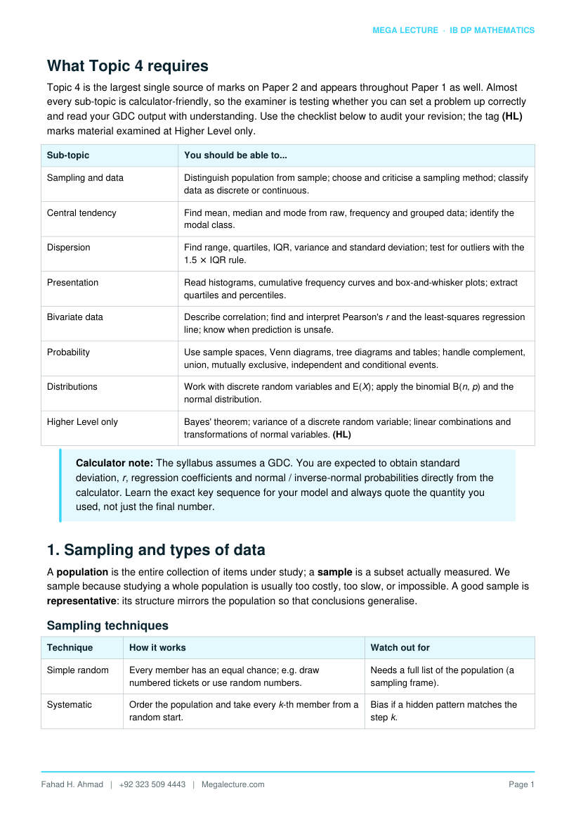
Topic 4 is the largest single source of marks on Paper 2 and appears throughout Paper 1 as well. Almost every sub-topic is calculator-friendly, so the examiner is testing whether you can set a problem up correctly and read your GDC output with understanding. Use the checklist below to audit your revision; the tag (HL) marks material examined at Higher Level only.

Sub-topic You should be able to...

Sampling and data Distinguish population from sample; choose and criticise a sampling method; classify data as discrete or continuous.

Central tendency Find mean, median and mode from raw, frequency and grouped data; identify the modal class.

Dispersion Find range, quartiles, IQR, variance and standard deviation; test for outliers with the 1.5 × IQR rule.

Presentation Read histograms, cumulative frequency curves and box-and-whisker plots; extract quartiles and percentiles.

Bivariate data Describe correlation; find and interpret Pearson's r and the least-squares regression line; know when prediction is unsafe.

Probability Use sample spaces, Venn diagrams, tree diagrams and tables; handle complement, union, mutually exclusive, independent and conditional events.

Distributions Work with discrete random variables and E(X); apply the binomial B(n, p) and the normal distribution.

Higher Level only Bayes' theorem; variance of a discrete random variable; linear combinations and transformations of normal variables. (HL)

Calculator note: The syllabus assumes a GDC. You are expected to obtain standard deviation, r, regression coefficients and normal / inverse-normal probabilities directly from the calculator. Learn the exact key sequence for your model and always quote the quantity you used, not just the final number.

1. Sampling and types of data

A population is the entire collection of items under study; a sample is a subset actually measured. We sample because studying a whole population is usually too costly, too slow, or impossible. A good sample is representative: its structure mirrors the population so that conclusions generalise.

Sampling techniques

Technique How it works Watch out for

Simple random Every member has an equal chance; e.g. draw numbered tickets or use random numbers.

Needs a full list of the population (a sampling frame).

Systematic Order the population and take every k-th member from a random start.

Bias if a hidden pattern matches the step k.

Technique How it works Watch out for

Stratified Split into groups (strata); sample each in proportion to its size.

Requires known strata sizes; must sample proportionally.

Quota Fill fixed numbers per category, but choose members non-randomly.

Interviewer choice introduces bias; not random.

Convenience Take whoever is easiest to reach. Usually unrepresentative; use only for rough pilots.

Reliability and bias

Bias is any systematic tendency for the sample to differ from the population (for example surveying only weekday-morning shoppers). Reliability concerns consistency: a reliable method gives similar results if repeated. A large sample reduces random error but does not remove bias — a biased method stays biased however many people you ask.

Even a random sample can mislead if the data-collection instrument is flawed. Non-response bias arises when those who do not reply differ from those who do; leading questions nudge respondents toward an answer; and a poorly chosen sampling frame may exclude part of the population entirely. Good practice is to pilot a questionnaire, keep questions neutral and unambiguous, and report the response rate.

Discrete vs continuous data

• Discrete data take separate, countable values (number of siblings, shoe size, goals scored).
• Continuous data can take any value in an interval and are limited only by the measuring instrument (height, mass, time).
• Discrete numerical data with many values are often grouped, after which they are handled with the same grouped-frequency tools as continuous data.

2. Measures of central tendency

A measure of central tendency is a single value that summarises the 'middle' of a data set. The three standard measures answer slightly different questions.

Measure Definition Best when...

Mean Sum of all values ÷ number of values. For frequency data, mean = (Σfx) / (Σf).

Data are roughly symmetric with no extreme outliers.

Median The middle value when data are ordered (average of the two middle values if n is even).

Data are skewed or contain outliers.

Mode The most frequent value; for grouped data, the modal class is the class of highest frequency.

Data are categorical, or the most typical value is wanted.

Grouped data and the modal class

With grouped data the individual values are lost, so we estimate the mean by assuming every value sits at its class mid-interval value (midpoint). The median is found from the cumulative frequency, and only the modal class — not a single modal value — can be named.

Effect of outliers

An outlier is an unusually large or small value. The mean is pulled toward an outlier because every value enters its calculation; the median and mode are resistant. This is why house prices and incomes, which are right-skewed, are usually reported with the median.

Worked example 1 — estimated mean and standard deviation of grouped data

The table shows the time (minutes) 30 students spent on homework one evening. Estimate the mean and the standard deviation.

Time [0,10): f=4; [10,20): f=8; [20,30): f=10; [30,40): f=6; [40,50): f=2.

Midpoints x = 5, 15, 25, 35, 45. Then Σfx = 5×4 + 15×8 + 25×10 + 35×6 + 45×2 = 20 + 120 + 250 + 210 + 90 = 690.

Estimated mean = 690 / 30 = 23.0 minutes. The modal class is [20, 30).

Σfx2 = 25×4 + 225×8 + 625×10 + 1225×6 + 2025×2 = 19550.

Variance = (Σfx2)/n − mean2 = 19550/30 − 23.02 = 651.67 − 529 = 122.67.

Standard deviation = √122.67 = 11.1 minutes (GDC: 1-Var Stats gives the same σn).

3. Measures of dispersion

Dispersion (spread) tells us how tightly the data cluster about the centre. Two data sets can share a mean yet differ hugely in spread, so a centre alone is never a complete summary.

Measure Definition / formula Comment

Range Largest value − smallest value. Quick but distorted by a single outlier.

Quartiles Q1, Q2 (median), Q3 split ordered data into four equal parts.

Read from the GDC or cumulative frequency.

Interquartile range IQR = Q3 − Q1 (the spread of the middle 50%). Resistant to outliers.

Variance Mean of the squared deviations from the mean. Units are squared.

Standard deviation σ σ = √variance (from the GDC). Same units as the data; the standard HL/SL measure.

Standard deviation in practice

The population standard deviation σ measures the typical distance of a value from the mean. You will read it directly from your GDC's one-variable statistics as σn; you are not expected to compute it by hand at SL, though you should recognise the formula variance = (Σf(x − mean)2) / n.

To compare the spread of two data sets with different means, the standard deviation (in the same units) is the usual choice; a larger σ means the values are, on average, further from their mean. Because every value enters its calculation, σ is itself sensitive to outliers, so quote it alongside the resistant IQR when the data may contain extreme values.

Identifying outliers: the 1.5 × IQR rule

A value is classified as an outlier if it lies

• below Q1 − 1.5×IQR (the lower fence), or
• above Q3 + 1.5×IQR (the upper fence).

Worked example 2 — quartiles, IQR and outliers

Ordered data: 3, 7, 8, 12, 14, 15, 18, 21, 22, 45 (n = 10). Find the median, the quartiles and the IQR, and test for outliers.

Median = average of 5th and 6th values = (14 + 15)/2 = 14.5.

Lower half 3, 7, 8, 12, 14 has median Q1 = 8; upper half 15, 18, 21, 22, 45 has median Q3 = 21. So IQR = 21 − 8 = 13.

Fences: lower = 8 − 1.5×13 = −11.5; upper = 21 + 1.5×13 = 40.5.

45 > 40.5, so 45 is an outlier; no value is below −11.5. The GDC returns the same Q1 = 8 and Q3 = 21.

Box-and-whisker plot of 4, 8, 9, 12, 14, 15, 18, 21, 24, 30. Five-number summary: min 4, Q1 9, median 14.5, Q3 21, max 30, so IQR = 12.

4. Presenting data

Marks are lost when candidates cannot read a diagram. Know exactly what each axis and feature represents.

Display What it shows Read from it

Frequency table Values / classes with their frequencies. Totals, mode, basis for all further calculation.

Histogram Continuous data as bars with no gaps; area (or height, equal widths) shows frequency.

Shape, modal class, skew.

Cumulative frequency curve

Running total of frequency plotted against the upper class boundary.

Median, quartiles, percentiles, number above / below a value.

Box-and-whisker plot Five-number summary: min, Q1, median, Q3, max. Spread, IQR, skew, outliers (if plotted separately).

Quartiles and percentiles from a cumulative frequency curve

For n data values, go up the cumulative-frequency axis to the required height, across to the curve, then down to the value axis:

• median (Q2) at height n/2; Q1 at n/4; Q3 at 3n/4.
• the p-th percentile at height pn/100 (e.g. the 90th percentile at 0.9n).

Exam tip: A box plot instantly reveals skew. If the median sits nearer Q1 (left box shorter) the data are positively (right) skewed; nearer Q3, negatively skewed. Symmetric data give a median in the middle of the box.

Histograms with unequal class widths

When classes have different widths, bar height must show frequency density = frequency ÷ class width, so that area represents frequency. Comparing raw heights of unequal-width bars is a common error. With equal widths, height and area tell the same story and either may be read directly.

Worked example 3 — reading a cumulative frequency curve

The marks of 80 students have cumulative frequencies ≤10 → 5, ≤20 → 18, ≤30 → 42, ≤40 → 66, ≤50 → 80. Estimate the median, the quartiles and the number scoring above 35.

Median = 40th value (n/2 = 40): it lies in 20–30, giving 20 + (40 − 18)/(42 − 18)×10 = 29.2.

Q1 = 20th value: 20 + (20 − 18)/24×10 = 20.8. Q3 = 60th value: 30 + (60 − 42)/24×10 = 37.5. IQR = 37.5 − 20.8 = 16.7.

At mark 35 the cumulative frequency is about 42 + (35 − 30)/10×(66 − 42) = 54, so roughly 80 − 54 = 26 students score above 35.

Cumulative frequency curve (ogive) for the 80 marks of Worked example 3. Reading across at n/2 = 40 gives the median ≈

29.2; at n/4 = 20 gives Q1 ≈ 20.8; at 3n/4 = 60 gives Q3 ≈ 37.5.

5. Bivariate data and correlation

Bivariate data are paired measurements (x, y) on each item. A scatter diagram plots the pairs and reveals any relationship. We describe an apparent linear relationship by its direction and strength.

Feature Description

Direction Positive: y rises as x rises. Negative: y falls as x rises. None: no trend.

Strength Strong (points close to a line) through to weak (widely scattered).

Pearson's product-moment correlation coefficient r

Pearson's r measures the strength and direction of a linear relationship, with −1 ≤ r ≤ +1. Values near ±1 mean a strong linear relationship; values near 0 mean a weak one. Read r straight from the GDC's linear-regression output.

|r| range Interpretation of the linear correlation

0.00 – 0.25 Very weak / none

0.25 – 0.50 Weak

0.50 – 0.75 Moderate

0.75 – 1.00 Strong (1 = perfect)

Correlation is not causation: A large |r| shows association, not that x causes y. Both may be driven by a third variable, or the link may be coincidental. Never claim causation from r alone.

Line of best fit and least-squares regression

The least-squares regression line of y on x is the straight line y = ax + b that minimises the sum of the squared vertical distances from the points to the line. The GDC returns a (gradient) and b (intercept). The line always passes through the mean point (mean of x, mean of y).

• Interpolation — predicting inside the range of the data — is reasonable, especially when |r| is large.
• Extrapolation — predicting outside the data range — is unreliable, because the linear pattern may not continue.

Use the line of y on x only to estimate y from x; it is not designed to estimate x from y.

Worked example 4 — correlation and the regression line

Five paired readings are (2, 5), (4, 8), (6, 10), (8, 13), (10, 15). Find Pearson's r and the least-squares line of y on x, then estimate y when x = 7.

The GDC gives r = 0.998 (a strong positive linear correlation) and y = 1.25x + 2.7 (gradient 1.25, intercept 2.7).

At x = 7, inside the data range 2–10, y = 1.25×7 + 2.7 = 11.45. This is interpolation, so with |r| so close to 1 the estimate is reliable.

Scatter plot of (2,5), (4,8), (6,10), (8,13), (10,15) with the least-squares regression line y = 2.70 + 1.25x drawn from the computed coefficients. Pearson r = 0.998 indicates a strong positive linear correlation; the open square marks the mean point.

6. Probability of events

An experiment has a set of possible outcomes called the sample space U; an event A is a subset of outcomes. For equally likely outcomes,

P(A) = n(A) / n(U), 0 ≤ P(A) ≤ 1.

The complement A′ is 'A does not happen', and

P(A′) = 1 − P(A).

Combined events

For any two events, the addition rule avoids double-counting the overlap:

P(A ∪ B) = P(A) + P(B) − P(A ∩ B).

Events are mutually exclusive if they cannot both occur, so P(A ∩ B) = 0 and the addition rule reduces to P(A ∪ B) = P(A) + P(B).

Independent events

Events are independent if one occurring does not change the probability of the other. Then the multiplication rule holds:

P(A ∩ B) = P(A) × P(B).

Conditional probability

The probability of A given that B has occurred is

P(A | B) = P(A ∩ B) / P(B), P(B) ≠ 0.

Rearranging gives the general multiplication rule P(A ∩ B) = P(B)×P(A | B), which is exactly what a tree diagram computes along its branches. Note that A and B are independent precisely when P(A | B) = P(A).

Mutually exclusive ≠ independent: These are different, and often opposite. If two events with non-zero probabilities are mutually exclusive, one happening forces the other to have probability 0 — that is maximum dependence, not independence.

Representing problems

• Venn diagrams handle overlap, union, complement and conditional questions on a fixed group.
• Tree diagrams suit sequential events; multiply along branches, add between paths, and remember branches change for 'without replacement'.
• Sample-space tables list all equally likely outcomes, ideal for two dice or two spinners.

Worked example 5 — Venn diagram

In a class of 30, 18 study French (F), 15 study Spanish (S) and 7 study both. Find (a) P(neither),

• P(French only), (c) P(F | S).

French only = 18 − 7 = 11; Spanish only = 15 − 7 = 8; both = 7; neither = 30 − (11 + 8 + 7) = 4.

• P(neither) = 4/30 = 2/15. (b) P(French only) = 11/30. (c) P(F | S) = P(F ∩ S)/P(S) = 7/15.

Worked example 6 — conditional probability with a tree

A bag holds 4 green and 3 yellow counters. Two are drawn without replacement. Find (a) P(both green), (b) P(the second is yellow), (c) P(the first was green given the second is yellow).

First draw: P(G) = 4/7, P(Y) = 3/7. Second-draw branches use the six counters that remain.

• P(G ∩ G) = (4/7)×(3/6) = 12/42 = 2/7.
• P(2nd Y) = P(G then Y) + P(Y then Y) = (4/7)×(3/6) + (3/7)×(2/6) = 12/42 + 6/42 = 18/42 = 3/7.
• P(1st G | 2nd Y) = P(G ∩ Y) / P(2nd Y) = (12/42) / (18/42) = 12/18 = 2/3.

Tree diagram for Worked example 6: two counters drawn without replacement from 4 green and 3 yellow. Branch probabilities are labelled and each node's branches sum to 1; the four path (joint) probabilities are shown at the leaves.

7. Discrete random variables

A discrete random variable X takes separate numerical values, each with a probability. A probability distribution lists the values with their probabilities, and these must satisfy

0 ≤ P(X = x) ≤ 1 and Σ P(X = x) = 1.

Expected value

The expected value (mean) is the long-run average value of X:

E(X) = Σ x P(X = x).

A game is called fair if its expected gain is 0. Setting up an unknown probability so that the probabilities sum to 1, or so that E(X) takes a required value, is a common exam task.

Worked example 7 — expected value of a game

A player pays $2 to roll a fair die and receives, in dollars, the number rolled. Find the expected gain per game and the entry fee that would make the game fair.

E(receipt) = (1 + 2 + 3 + 4 + 5 + 6)/6 = 3.5, so expected gain = 3.5 − 2 = +$1.50 (the game favours the player).

The game is fair when the fee equals E(receipt) = $3.50.

Variance of a discrete random variable (HL)

(HL) The spread of X is measured by its variance

Var(X) = E(X2) − [E(X)]2, where E(X2) = Σ x2 P(X = x).

(HL) The standard deviation of X is √Var(X). Be careful: E(X2) is not [E(X)]2.

Worked example 8 — expected value and variance (HL)

X has distribution P(0)=0.1, P(1)=0.3, P(2)=0.4, P(3)=0.2. Find E(X) and Var(X).

Check: 0.1 + 0.3 + 0.4 + 0.2 = 1. Good.

E(X) = 0×0.1 + 1×0.3 + 2×0.4 + 3×0.2 = 0 + 0.3 + 0.8 + 0.6 = 1.7.

E(X2) = 0 + 1×0.3 + 4×0.4 + 9×0.2 = 0.3 + 1.6 + 1.8 = 3.7.

Var(X) = 3.7 − 1.72 = 3.7 − 2.89 = 0.81 (so SD = √0.81 = 0.9). (HL)

8. The binomial distribution B(n, p)

The binomial distribution counts the number of successes X in a fixed number of trials. Write X ~ B(n, p). The four conditions must all hold:

• a fixed number n of trials;
• each trial has just two outcomes, success or failure;
• the probability of success p is constant;
• the trials are independent.

The probability of exactly x successes is

P(X = x) = nCx px (1 − p)n−x, x = 0, 1, ..., n, where nCx = n! / [x!(n−x)!] is the binomial coefficient (Topic 1). Its mean and variance are mean = np, variance = np(1 − p).

In practice use the GDC: binompdf(n, p, x) for P(X = x) and binomcdf(n, p, x) for P(X ≤ x). Translate the words carefully: 'at least one' = 1 − P(X = 0), 'more than 3' = 1 − P(X ≤ 3).

The distribution is symmetric only when p = 0.5; for small p it is right-skewed and for large p left-skewed. Because each trial must be independent with constant p, sampling without replacement from a small population is not binomial — the probability changes from draw to draw. It is acceptable only as an approximation when the sample is a tiny fraction of a very large population.

Worked example 9 — binomial distribution

A machine produces components, each independently defective with probability 0.10. A sample of 12 is taken. Find (a) P(exactly 2 defective), (b) P(at least one defective), and (c) the mean and variance of the number defective.

Here X ~ B(12, 0.10).

• P(X = 2) = 12C2 (0.10)2(0.90)10 = 66 × 0.01 × 0.34868 = 0.230 (3 s.f.).
• P(X ≥ 1) = 1 − P(X = 0) = 1 − (0.90)12 = 1 − 0.28243 = 0.718.
• Mean = np = 12×0.10 = 1.2; variance = np(1−p) = 12×0.10×0.90 = 1.08.

Binomial distribution B(12, 0.10) from Worked example 9. Each bar height equals P(X = k) = 12Ck(0.10)k(0.90)12−k; the marked bar is P(X = 2) = 0.230.

9. The normal distribution

The normal distribution models continuous data that cluster symmetrically about a mean, such as heights or measurement errors. Write X ~ N(μ, σ2), with mean μ and standard deviation σ.

Key properties

• The curve is bell-shaped and symmetric about x = μ; the total area under it is 1, so P(X < μ) = 0.5.
• Mean, median and mode all equal μ.
• About 68% of data lie within 1σ of the mean, 95% within 2σ, and 99.7% within 3σ (the 68–95–99.7 rule).

Standardising

Any normal variable is converted to the standard normal Z ~ N(0, 1) by z = (x − μ) / σ.

The z-score states how many standard deviations x lies above (positive) or below (negative) the mean, and lets you compare values from different normal distributions. On the GDC use normalcdf(lower, upper, μ, σ) for a probability, and invNorm(area, μ, σ) for the inverse problem — finding the value with a given probability below it.

Worked example 10 — normal probabilities and inverse normal

Adult heights are modelled by X ~ N(170, 82) cm. Find (a) P(X < 180), (b) P(165 < X < 175), (c) the height exceeded by 90% of adults.

• z = (180 − 170)/8 = 1.25, so P(X < 180) = P(Z < 1.25) = 0.894.
• z-scores ±0.625, so P = normalcdf(165, 175, 170, 8) = 0.468.
• 'Exceeded by 90%' means P(X > h) = 0.90, i.e. P(X < h) = 0.10. Then h = invNorm(0.10, 170,
• = 170 + (−1.2816)×8 = 170 − 10.25 = 159.75 ≈ 160 cm.

Normal distribution N(μ, σ2) for adult heights with μ = 170 cm and σ = 8 cm. The shaded region is P(X < 180) = 0.894, matching Worked example 10(a).

Standardising pitfalls: Divide by σ, not σ2 (the notation N(μ, σ2) quotes the variance, but the formula uses σ). Sketch the bell and shade the region so you know whether to use the area to the left, to the right, or between two values.

Finding an unknown mean or standard deviation

If a probability is given but μ or σ is unknown, work backwards through the z-score. First find the z-value for the stated probability with invNorm(area, 0, 1); then substitute into z = (x − μ)/σ and solve. For example, if 20% of values exceed 60 and σ = 10, then invNorm(0.80, 0, 1) = 0.8416, so 0.8416 = (60 − μ)/10, giving μ = 60 − 8.416 = 51.6. Two unknowns require two such equations solved simultaneously.

10. Bayes' theorem (HL)

(HL) Bayes' theorem reverses a conditional probability: it finds P(A | B) when you know P(B | A). For an event partitioned by A and its complement A′,

P(A | B) = [P(A)P(B | A)] / [P(A)P(B | A) + P(A′)P(B | A′)].

(HL) The denominator is just P(B) expanded by the law of total probability — the sum of the two tree paths that reach B. The syllabus also states the theorem for a partition into three events; the pattern is the same, with three terms in the denominator.

Worked example 11 — Bayes' theorem (HL)

A disease affects 1% of a population. A test is 95% likely to be positive for someone with the disease, but also gives a positive result for 10% of healthy people. A person tests positive. Find the probability they actually have the disease.

Let D = has disease, so P(D) = 0.01, P(D′) = 0.99. P(+ | D) = 0.95, P(+ | D′) = 0.10.

P(+) = P(D)P(+ | D) + P(D′)P(+ | D′) = 0.01×0.95 + 0.99×0.10 = 0.0095 + 0.099 = 0.1085.

P(D | +) = 0.0095 / 0.1085 = 0.0876 (about 8.8%).

The result is surprisingly low: because the disease is rare, most positives are false positives from the large healthy group. This 'base-rate' insight is the point of the example. (HL)

11. Combining random variables (HL)

(HL) Scaling and shifting a random variable follow simple rules. For constants a and b,

E(aX + b) = aE(X) + b, Var(aX + b) = a2Var(X).

(HL) Adding a constant b shifts the mean but leaves the spread unchanged; multiplying by a scales the standard deviation by |a| and the variance by a2.

Linear transformations of a normal variable (HL)

(HL) A linear function of a normal variable is itself normal: if X ~ N(μ, σ2) then aX + b ~ N(aμ + b, a2σ2).

(HL) Standardising, z = (x − μ)/σ, is exactly this transformation with a = 1/σ and b = −μ/σ, which is why the result is the standard normal N(0, 1). For independent normal variables X and Y, the sum and difference are also normal, with means μX ± μY and variance σX

2 + σY 2 in both cases (variances always add for independent variables).

(HL) Example: if X has mean 4 and variance 3, then Y = 2X − 1 has mean 2×4 − 1 = 7 and variance 22×3 = 12 (standard deviation √12 ≈ 3.46). Notice the −1 shifts the mean but does not affect the spread.

12. Common pitfalls

• Confusing mutually exclusive (cannot co-occur, P(A ∩ B) = 0) with independent (no influence, P(A ∩ B) = P(A)P(B)).
• Inverting the conditional: P(A | B) is not P(B | A). Divide by the probability of the given event.
• Using nCx for order-dependent counts, or forgetting it entirely in the binomial formula.
• Standardising with the variance instead of the standard deviation, or losing the sign of a negative z-score.
• Extrapolating a regression line far beyond the data, or using the y-on-x line to predict x.
• Forgetting that branches change on a 'without replacement' tree, or treating a grouped-data mean as exact rather than an estimate.
• Claiming causation from a correlation coefficient.

13. Quick-reference formulae

Quantity Formula

Mean (frequency data) mean = (Σfx) / (Σf)

Interquartile range IQR = Q3 − Q1

Outlier fences below Q1 − 1.5×IQR or above Q3 + 1.5×IQR

Standard deviation σ = √variance (from the GDC)

Complement P(A′) = 1 − P(A)

Addition (union) P(A ∪ B) = P(A) + P(B) − P(A ∩ B)

Independent events P(A ∩ B) = P(A)×P(B)

Conditional P(A | B) = P(A ∩ B) / P(B)

Expected value E(X) = Σ x P(X = x)

Variance of X (HL) Var(X) = E(X2) − [E(X)]2

Binomial B(n, p) P(X=x) = nCx px(1−p)n−x; mean np, var np(1−p)

Standardising z = (x − μ) / σ

Bayes (HL) P(A|B) = P(A)P(B|A) / P(B)

Linear transform (HL) E(aX+b) = aE(X)+b; Var(aX+b) = a2Var(X)

14. Test yourself

Attempt all ten without notes, then check against the full worked answers that follow. Questions marked (HL) are Higher Level only.

• A school of 1200 students has year groups of 400, 300, 300 and 200. Explain how to take a stratified sample of 60 students.
• Homework times (minutes) are grouped: [0,5) 3, [5,10) 9, [10,15) 14, [15,20) 10, [20,25) 4. State the modal class and estimate the mean.
• Data: 12, 15, 15, 18, 20, 22, 25, 28, 31, 55. Find the median, Q1, Q3 and IQR, and test 55 for being an outlier.
• For a data set, r = 0.92 and the regression line is y = 2.3x + 5 (data for 2 ≤ x ≤ 9). Describe the correlation, predict y when x = 6, and comment on predicting y when x = 30.
• P(A) = 0.5, P(B) = 0.4, P(A ∪ B) = 0.7. Find P(A ∩ B). Are A and B independent? Mutually exclusive?
• One card is drawn from a standard pack of 52. Let A = 'a heart' and B = 'a king'. Are A and B independent?
• 60% of students travel by bus, of whom 20% are late; the other 40% walk, of whom 10% are late. A student is late. Find the probability they came by bus.
• X ~ B(8, 0.3). Find P(X = 3) and the mean of X.
• Test scores are X ~ N(50, 52). Find P(X > 58) and the score exceeded by only 5% of candidates.
• (HL) X takes values 1, 2, 3, 4 with probabilities 0.4, 0.3, 0.2, 0.1. Find E(X) and Var(X).

Worked answers

• Sampling fraction = 60/1200 = 1/20, so take 1/20 of each year: 20, 15, 15 and 10 students. Within each year select at random (e.g. random numbers on a class list) so every student has an equal chance.
• Modal class = [10, 15) (highest frequency 14). Midpoints 2.5, 7.5, 12.5, 17.5, 22.5; Σfx = 7.5 + 67.5 + 175 + 175 + 90 = 515; n = 40. Estimated mean = 515/40 = 12.875 ≈ 12.9 min.
• Median = (20 + 22)/2 = 21. Lower half 12, 15, 15, 18, 20 gives Q1 = 15; upper half 22, 25, 28, 31, 55 gives Q3 = 28; IQR = 13. Upper fence = 28 + 1.5×13 = 47.5; since 55 > 47.5, 55 is an outlier.
• r = 0.92 is a strong positive linear correlation. At x = 6 (inside the data), y = 2.3×6 + 5 = 18.8. At x = 30 the prediction is unreliable — that is extrapolation far outside the data range 2 to 9, where the linear trend may not hold.
• P(A ∩ B) = P(A) + P(B) − P(A ∪ B) = 0.5 + 0.4 − 0.7 = 0.2. Since P(A)P(B) = 0.5×0.4 = 0.2 = P(A ∩ B), the events are independent. They are not mutually exclusive, because P(A ∩ B) ≠ 0.
• P(A) = 13/52 = 1/4, P(B) = 4/52 = 1/13, and P(A ∩ B) (king of hearts) = 1/52. Since (1/4)×(1/13) = 1/52 = P(A ∩ B), the events are independent.
• P(late) = 0.6×0.2 + 0.4×0.1 = 0.12 + 0.04 = 0.16. P(bus | late) = 0.12/0.16 = 0.75.
• P(X = 3) = 8C3(0.3)3(0.7)5 = 56×0.027×0.16807 = 0.254. Mean = np = 8×0.3 = 2.4.
• z = (58 − 50)/5 = 1.6, so P(X > 58) = P(Z > 1.6) = 0.0548. For the top 5%, invNorm(0.95, 50, 5) = 50 + 1.645×5 = 58.2.
• (HL) E(X) = 1×0.4 + 2×0.3 + 3×0.2 + 4×0.1 = 0.4 + 0.6 + 0.6 + 0.4 = 2.0. E(X2) = 1×0.4 + 4×0.3 + 9×0.2 + 16×0.1 = 0.4 + 1.2 + 1.8 + 1.6 = 5.0. Var(X) = 5.0 − 2.02 = 1.0.