A Level Accounting: cost and management accounting notes

These revision notes cover the A Level (Paper 3) cost and management accounting content of the Cambridge International AS & A Level Accounting syllabus (9706). There are four topics: activity-based costing, budgeting and budgetary control, standard costing and variance analysis, and investment appraisal. Every business and every figure is invented for these notes. Each worked example shows all of its steps and has been checked so that its totals agree. The notes finish with a glossary, a set of short questions and three longer structured questions in the style of Paper 3. All of them have answers and mark allocations.

1. Activity-based costing (ABC)

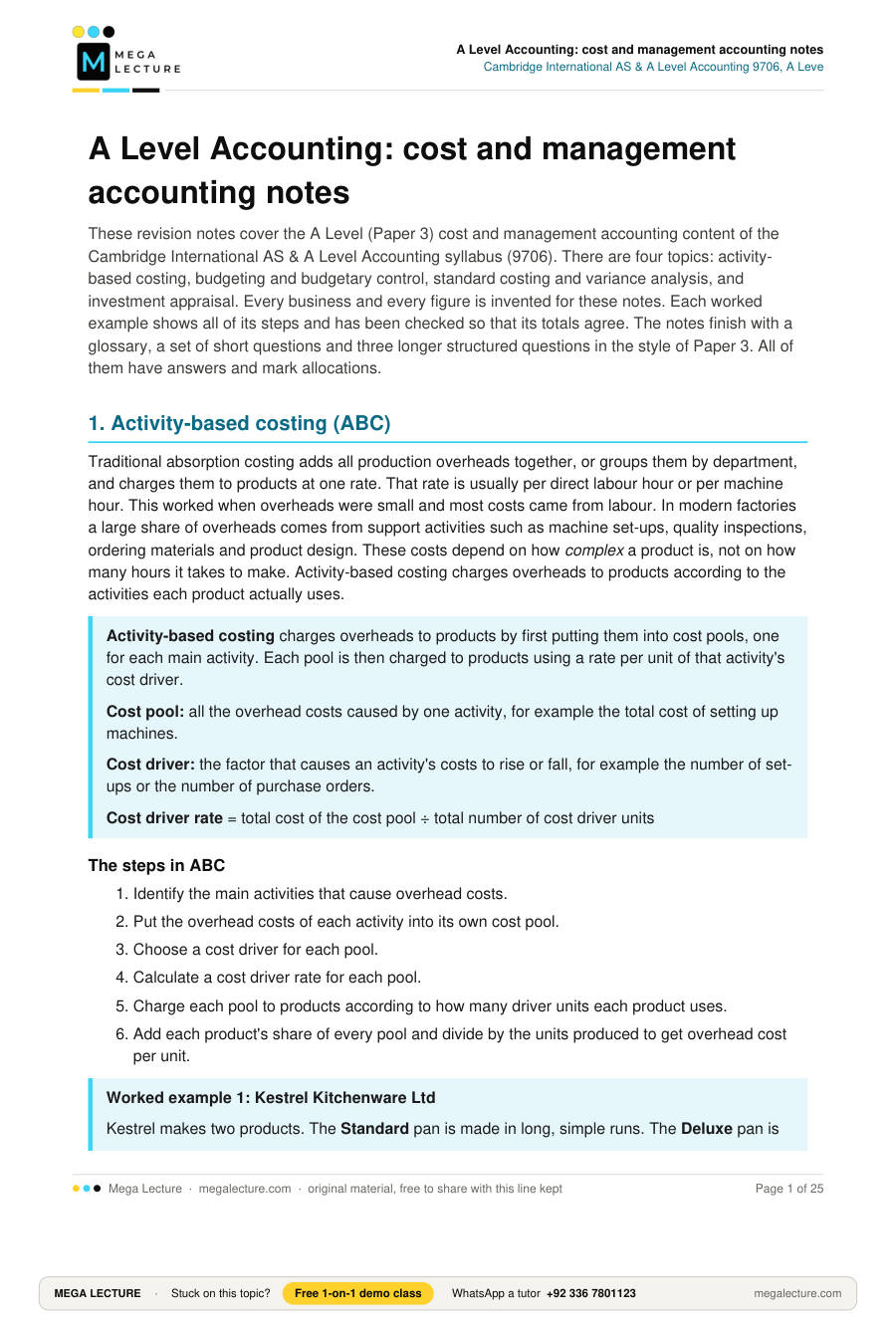
Traditional absorption costing adds all production overheads together, or groups them by department, and charges them to products at one rate. That rate is usually per direct labour hour or per machine hour. This worked when overheads were small and most costs came from labour. In modern factories a large share of overheads comes from support activities such as machine set-ups, quality inspections, ordering materials and product design. These costs depend on how complex a product is, not on how many hours it takes to make. Activity-based costing charges overheads to products according to the activities each product actually uses.

Activity-based costing charges overheads to products by first putting them into cost pools, one for each main activity. Each pool is then charged to products using a rate per unit of that activity's cost driver.

Cost pool: all the overhead costs caused by one activity, for example the total cost of setting up machines.

Cost driver: the factor that causes an activity's costs to rise or fall, for example the number of set-ups or the number of purchase orders.

Cost driver rate = total cost of the cost pool ÷ total number of cost driver units

The steps in ABC

1. Identify the main activities that cause overhead costs.
2. Put the overhead costs of each activity into its own cost pool.
3. Choose a cost driver for each pool.
4. Calculate a cost driver rate for each pool.
5. Charge each pool to products according to how many driver units each product uses.
6. Add each product's share of every pool and divide by the units produced to get overhead cost per unit.

Worked example 1: Kestrel Kitchenware Ltd

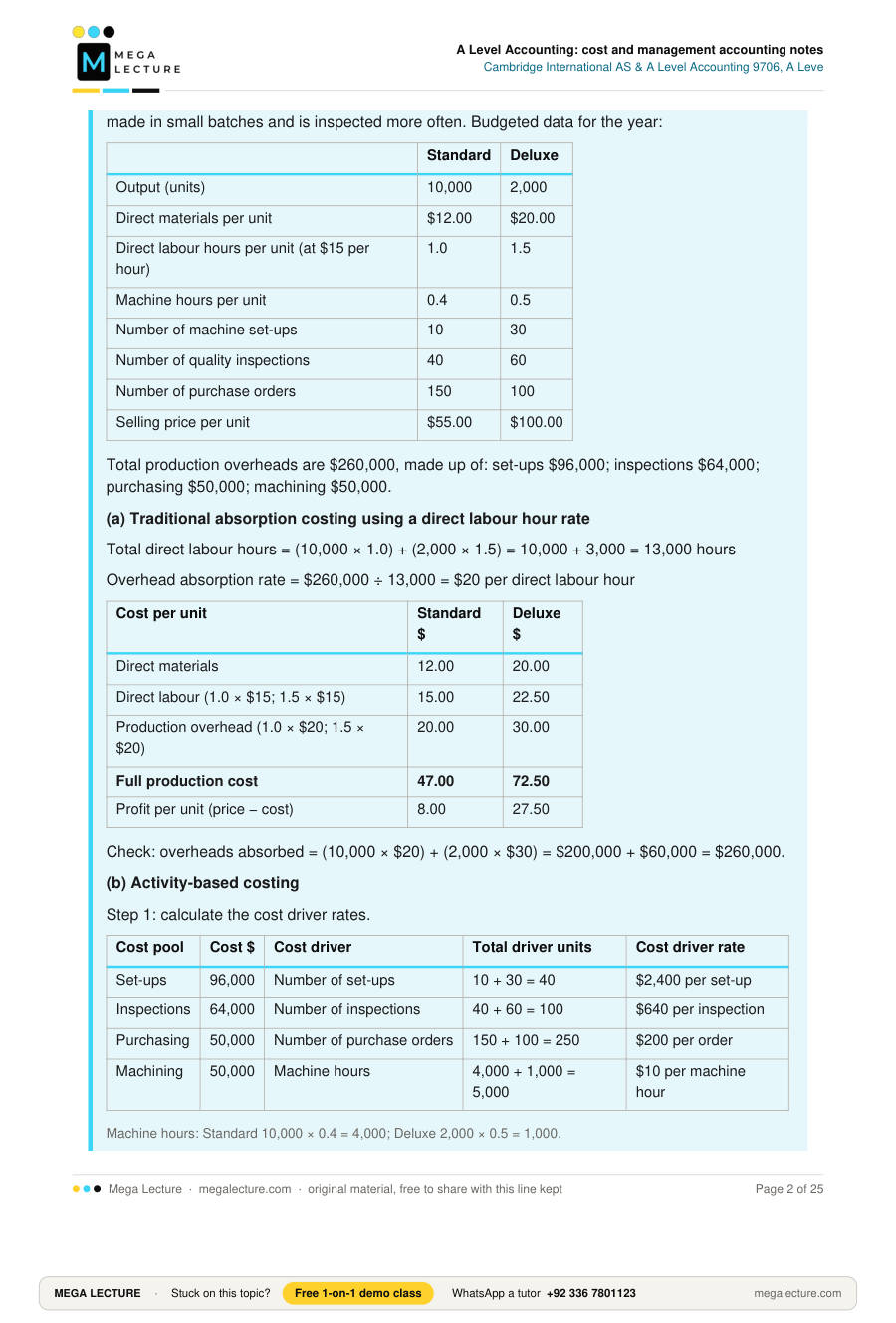
Kestrel makes two products. The Standard pan is made in long, simple runs. The Deluxe pan is made in small batches and is inspected more often. Budgeted data for the year:

Standard	Deluxe
Output (units)	10,000	2,000
Direct materials per unit	$12.00	$20.00
Direct labour hours per unit (at $15 per hour)	1.0	1.5
Machine hours per unit	0.4	0.5
Number of machine set-ups	10	30
Number of quality inspections	40	60
Number of purchase orders	150	100
Selling price per unit	$55.00	$100.00

Total production overheads are $260,000, made up of: set-ups $96,000; inspections $64,000; purchasing $50,000; machining $50,000.

(a) Traditional absorption costing using a direct labour hour rate

Total direct labour hours = (10,000 × 1.0) + (2,000 × 1.5) = 10,000 + 3,000 = 13,000 hours

Overhead absorption rate = $260,000 ÷ 13,000 = $20 per direct labour hour

Cost per unit	Standard $	Deluxe $
Direct materials	12.00	20.00
Direct labour (1.0 × $15; 1.5 × $15)	15.00	22.50
Production overhead (1.0 × $20; 1.5 × $20)	20.00	30.00
Full production cost	47.00	72.50
Profit per unit (price − cost)	8.00	27.50

Check: overheads absorbed = (10,000 × $20) + (2,000 × $30) = $200,000 + $60,000 = $260,000.

(b) Activity-based costing

Step 1: calculate the cost driver rates.

Cost pool	Cost $	Cost driver	Total driver units	Cost driver rate
Set-ups	96,000	Number of set-ups	10 + 30 = 40	$2,400 per set-up
Inspections	64,000	Number of inspections	40 + 60 = 100	$640 per inspection
Purchasing	50,000	Number of purchase orders	150 + 100 = 250	$200 per order
Machining	50,000	Machine hours	4,000 + 1,000 = 5,000	$10 per machine hour

Machine hours: Standard 10,000 × 0.4 = 4,000; Deluxe 2,000 × 0.5 = 1,000.

Step 2: charge each pool to the two products.

Cost pool	Standard $	Deluxe $	Total $
Set-ups (10 × $2,400; 30 × $2,400)	24,000	72,000	96,000
Inspections (40 × $640; 60 × $640)	25,600	38,400	64,000
Purchasing (150 × $200; 100 × $200)	30,000	20,000	50,000
Machining (4,000 × $10; 1,000 × $10)	40,000	10,000	50,000
Total overhead	119,600	140,400	260,000
Units produced	10,000	2,000
Overhead per unit	11.96	70.20

Step 3: find the full cost and profit per unit.

Cost per unit	Standard $	Deluxe $
Direct materials	12.00	20.00
Direct labour	15.00	22.50
Production overhead (ABC)	11.96	70.20
Full production cost	38.96	112.70
Profit/(loss) per unit	16.04	(12.70)

Comment: Absorption costing charged the Deluxe pan only $30 of overhead per unit. This is because overhead was charged by labour hours, and labour hours do not reflect the set-ups and inspections the Deluxe pan causes: it used only 3,000 of the 13,000 labour hours. ABC charges $70.20, because the Deluxe pan causes 75% of the set-ups and 60% of the inspections even though it is only one-sixth of output. Under absorption costing the Deluxe pan looked like the more profitable product per unit ($27.50 against $8.00). ABC shows that each Deluxe pan is sold at a loss of $12.70, while the Standard pan was being over-costed. Managers could raise the Deluxe price, cut the number of Deluxe batches, or reconsider the product altogether. Before dropping it they should check how much of the $140,400 would really be saved, because some activity costs may be fixed in the short run.

ABC compared with traditional absorption costing

Feature	Traditional absorption costing	Activity-based costing
Grouping of overheads	By production department or cost centre	By activity (cost pool)
Basis of charging	Usually volume-based: labour or machine hours	Cost drivers, which are often transactions such as set-ups or orders
Number of rates	One per department, sometimes one for the whole factory	One per activity, so usually many
Treatment of low-volume, complex products	Tends to under-cost them	Charges them their full share of support costs
Treatment of high-volume, simple products	Tends to over-cost them	Usually gives a lower, more realistic cost
Cost of running the system	Lower and simpler	Higher, because activity data must be collected

Advantages of ABC

• It gives more accurate product costs when overheads are a large share of total cost and products differ in complexity.
• Pricing decisions are better, which makes it less likely that products are sold below their true cost.
• Managers can see what causes overheads, so the activities that drive costs can be reduced. For example, fewer set-ups can be achieved by making larger batches.
• Profitability analysis by product or customer is more reliable.
• It suits modern automated businesses and service businesses, where direct labour is a small share of total cost.

Limitations of ABC

• It is time-consuming and expensive to set up and to keep running.
• Choosing cost pools and drivers takes judgement, and some costs, such as factory rent, have no clear activity driver and still have to be apportioned arbitrarily.
• A cost pool may have more than one driver, but ABC uses only one.
• The benefit is small when overheads are low or when products are similar.
• ABC costs are still based on past or budgeted data. They are not always relevant costs for short-term decisions.

Link to IAS 2 Inventories: inventory in published financial statements must include a share of production overheads, allocated systematically on the basis of normal capacity. Non-production overheads such as selling costs must be excluded. ABC is mainly a tool for internal management decisions and does not replace the IAS 2 rules for valuing inventory.

2. Budgeting and budgetary control

Budget: a detailed plan for a future period, expressed in money and/or quantities, that the business intends to achieve.

Budgetary control: setting budgets that make managers responsible for their areas, regularly comparing actual results with the budget, and acting on the differences (variances).

Principal budget factor (limiting factor): the factor that limits the activity of the business, usually sales demand. The budget for this factor must be prepared first.

Purposes of budgeting

• Planning: managers must think ahead and spot problems early, such as a cash shortage.
• Co-ordination: the sales, production, purchasing and finance plans are made to fit together.
• Communication: every manager learns what is expected of them.
• Control: actual results can be measured against a target.
• Motivation: targets that are demanding but achievable can improve performance.
• Responsibility: each budget holder is accountable for their own costs or revenue.

Order of preparation of functional budgets

When sales is the principal budget factor, the budgets are prepared in this order: sales budget → production budget → materials usage budget → materials purchases budget → labour budget → overhead budgets → cash budget → budgeted income statement → budgeted statement of financial position. The cash budget, budgeted income statement and budgeted statement of financial position together form the master budget.

Key formulae

Production (units) = budgeted sales + closing inventory of finished goods − opening inventory of finished goods

Materials purchases (quantity) = materials used in production + closing inventory of materials − opening inventory of materials

Labour cost = units produced × hours per unit × rate per hour

Worked example 2: Zarrar Components Ltd — functional budgets

Zarrar makes one product, a water-pump housing, which sells for $40. Budgeted sales in units are: January 2,000; February 2,400; March 3,000; April 2,600. December sales were 1,800 units.

• Closing inventory of finished goods each month is 20% of the next month's sales. The opening inventory on 1 January follows the same policy.
• Each unit needs 3 kg of material at $5 per kg. Closing inventory of materials is 25% of the next month's usage, and the opening inventory on 1 January follows the same policy. April production is budgeted at 2,560 units.
• Each unit takes 0.5 direct labour hours at $16 per hour.

Sales budget

January	February	March
Units	2,000	2,400	3,000
Revenue at $40 ($)	80,000	96,000	120,000

Production budget (units)

January	February	March
Budgeted sales	2,000	2,400	3,000
Add closing inventory (20% of next month)	480	600	520
Less opening inventory	(400)	(480)	(600)
Production	2,080	2,520	2,920

January opening inventory = 20% × 2,000 = 400 units. March closing inventory = 20% × April sales of 2,600 = 520 units.

Materials usage and purchases budget

January	February	March
Usage (production × 3 kg)	6,240	7,560	8,760
Add closing inventory (25% of next month's usage)	1,890	2,190	1,920
Less opening inventory	(1,560)	(1,890)	(2,190)
Purchases (kg)	6,570	7,860	8,490
Purchases at $5 per kg ($)	32,850	39,300	42,450

April usage = 2,560 × 3 = 7,680 kg, so March closing inventory = 25% × 7,680 = 1,920 kg. January opening inventory = 25% × 6,240 = 1,560 kg.

Direct labour budget

January	February	March
Production (units)	2,080	2,520	2,920
Hours (× 0.5)	1,040	1,260	1,460
Cost at $16 per hour ($)	16,640	20,160	23,360

The cash budget

A cash budget shows the expected cash receipts and payments in each period and the closing bank balance. It includes only cash items, recorded in the period when the cash moves. Leave out depreciation, bad debts written off, provisions and any other non-cash item. Include capital items such as buying a machine, receiving a loan or issuing shares, because they involve cash.

Worked example 3: Zarrar Components Ltd — cash budget for January to March

Additional information:

• 30% of sales are for cash. The other 70% are on credit and are received in the month after the sale. December sales were 1,800 units at $40 = $72,000.
• Materials are paid for in the month after purchase. December purchases were $30,000.
• Wages are paid in the month they are earned.
• Fixed overheads are $18,000 a month. This includes $3,000 of depreciation. The rest is paid in the month it is incurred.
• A new machine costing $40,000 will be paid for in February.
• The bank balance on 1 January is $12,000.

January $	February $	March $
Receipts
Cash sales (30% of this month)	24,000	28,800	36,000
Credit customers (70% of last month)	50,400	56,000	67,200
Total receipts	74,400	84,800	103,200
Payments
Materials (last month's purchases)	30,000	32,850	39,300
Wages	16,640	20,160	23,360
Fixed overheads ($18,000 − $3,000)	15,000	15,000	15,000
Machine	–	40,000	–
Total payments	61,640	108,010	77,660
Net cash flow	12,760	(23,210)	25,540
Opening balance	12,000	24,760	1,550
Closing balance	24,760	1,550	27,090

Comment: The bank balance falls to only $1,550 at the end of February because the machine is bought in the same month that production, and therefore wages, rises. A small delay in receiving money from customers could leave the account overdrawn. Zarrar could arrange an overdraft facility in advance, lease the machine, pay for it in instalments, or buy it in March instead.

The master budget

The master budget brings all the functional budgets together into a budgeted income statement and a budgeted statement of financial position, along with the cash budget. The budgeted profit is usually different from the change in cash. The example below shows why.

Worked example 4: Zarrar Components Ltd — budgeted income statement and budgeted statement of financial position

Inventory is valued at variable production cost: materials $15 + labour $8 = $23 per unit.

Marginal (variable) cost is used here because the budget is for internal planning. For published financial statements, IAS 2 would require a share of fixed production overheads to be included in the inventory value.

(a) Budgeted income statement for the quarter ending 31 March

$	$
Revenue (7,400 units × $40)	296,000
Opening inventory of finished goods (400 × $23)	9,200
Materials used (22,560 kg × $5)	112,800
Direct labour	60,160
Less closing inventory of finished goods (520 × $23)	(11,960)
Cost of sales	(170,200)
Contribution	125,800
Fixed overheads including depreciation (3 × $18,000)	(54,000)
Budgeted profit for the quarter	71,800

Check: cost of sales = 7,400 units × $23 = $170,200.

(b) Budgeted statement of financial position at 31 March

On 1 January Zarrar's non-current assets had a net book value of $180,000 and its share capital was $160,000. The other opening balances come from worked examples 2 and 3. Tax and dividends are ignored.

1 January (actual) $	31 March (budget) $
Non-current assets at net book value	180,000	211,000
Current assets
Inventory of materials (1,560 kg; 1,920 kg × $5)	7,800	9,600
Inventory of finished goods (400; 520 units × $23)	9,200	11,960
Trade receivables (70% of December; 70% of March sales)	50,400	84,000
Bank	12,000	27,090
Total current assets	79,400	132,650
Total assets	259,400	343,650
Equity
Share capital	160,000	160,000
Retained earnings	69,400	141,200
Total equity	229,400	301,200
Current liabilities
Trade payables (December; March purchases)	30,000	42,450
Total equity and liabilities	259,400	343,650

Workings: non-current assets = $180,000 + machine $40,000 − depreciation (3 × $3,000) $9,000 = $211,000. Retained earnings = $69,400 + budgeted profit $71,800 = $141,200. There are no accruals, because wages and cash overheads are paid in the month they are incurred.

(c) Why does profit of $71,800 lead to only $15,090 more cash ($12,000 → $27,090)?

$
Budgeted profit	71,800
Add back depreciation (non-cash)	9,000
Machine purchased	(40,000)
Increase in trade receivables ($50,400 → $84,000)	(33,600)
Increase in trade payables ($30,000 → $42,450)	12,450
Increase in materials inventory (1,560 kg → 1,920 kg at $5)	(1,800)
Increase in finished goods inventory ($9,200 → $11,960)	(2,760)
Increase in cash	15,090

Every figure in this reconciliation is a change between the two columns of the statement of financial position, so the three parts of the master budget agree with each other.

Fixed and flexible budgets

A fixed budget is set for one planned level of activity and does not change if actual activity is different. Comparing actual results with a fixed budget can mislead: if output is 10% below budget, costs will look "favourable" just because fewer units were made.

Flexible budget: a budget that is adjusted to the actual level of activity. Variable costs and revenue are flexed in proportion to activity, and fixed costs stay the same. It allows like-for-like comparison with actual results.

Worked example 5: Orchid Furniture — flexing a budget

Orchid budgeted to make and sell 5,000 chairs but actually made and sold 4,400. The budget per chair is: selling price $60, materials $14, labour $10, variable overhead $6. Fixed overheads are budgeted at $60,000.

Original budget (5,000) $	Flexed budget (4,400) $	Actual (4,400) $	Variance $
Revenue	300,000	264,000	272,800	8,800 F
Direct materials	(70,000)	(61,600)	(64,300)	2,700 A
Direct labour	(50,000)	(44,000)	(42,900)	1,100 F
Variable overhead	(30,000)	(26,400)	(27,100)	700 A
Fixed overhead	(60,000)	(60,000)	(61,500)	1,500 A
Profit	90,000	72,000	77,000	5,000 F

The variance column compares actual results with the flexed budget. F = favourable (it increases profit); A = adverse (it reduces profit).

Analysis: Profit was $13,000 below the original budget ($90,000 − $77,000). Selling 600 fewer chairs cost $18,000 of profit, which is the difference between the original and flexed budgets (600 × $30 contribution per chair). Selling price and cost performance at the actual level of activity were $5,000 better than planned. Check: $18,000 A − $5,000 F = $13,000 A. Actual revenue per chair was $272,800 ÷ 4,400 = $62. The higher price may explain why fewer chairs were sold.

Behavioural aspects of budgeting

• Participation (bottom-up budgeting): managers who help set their own budgets are more likely to accept and work towards them. This takes more time and invites budgetary slack.
• Imposed (top-down) budgets: these are quicker to set and match the company's overall objectives. Staff may resent them and feel little ownership.
• Budgetary slack: managers may overstate costs or understate revenue so that their targets are easy to hit.
• Target difficulty: targets that are too easy do not motivate. Targets that seem impossible cause staff to give up.
• "Spend it or lose it": managers may spend unused budget near the year end so that next year's allowance is not cut.
• Short-termism and goal incongruence: a manager may cut training or maintenance to meet this year's cost budget, which harms the business in the long run.
• Blame culture: if budgets are used mainly to punish adverse variances, managers may hide problems or manipulate figures.

Limitations of budgeting

• Budgets are based on forecasts, which may turn out to be wrong, for example because of inflation, exchange rates or competitors' actions.
• They take time and cost money to prepare.
• They can be rigid and discourage managers from responding to new opportunities.
• Incremental budgeting, which adds a percentage to last year's figures, carries past inefficiencies forward.
• Non-financial matters such as quality and customer satisfaction may be ignored.

3. Standard costing and variance analysis

Standard cost: the planned cost of one unit of product, built up from standard quantities of materials and labour at standard prices and rates, plus overheads at standard absorption rates.

Variance: the difference between a standard (or budgeted) figure and the actual figure. A favourable variance increases profit and an adverse variance reduces it.

Types of standard: an ideal standard assumes perfect conditions with no waste or idle time. An attainable standard allows for normal waste and breakdowns and is the best for motivation. A basic standard is left unchanged over long periods and is used to show trends.

Variance formulae

Variance	Formula
Material price	(Standard price − actual price) × actual quantity purchased/used
Material usage	(Standard quantity for actual output − actual quantity used) × standard price
Labour rate	(Standard rate − actual rate) × actual hours paid
Labour efficiency	(Standard hours for actual output − actual hours worked) × standard rate
Variable overhead expenditure	(Actual hours × standard variable overhead rate) − actual variable overhead
Variable overhead efficiency	(Standard hours for actual output − actual hours) × standard variable overhead rate
Fixed overhead expenditure	Budgeted fixed overhead − actual fixed overhead
Fixed overhead volume	(Actual output − budgeted output) × standard fixed overhead per unit
Sales price	(Actual selling price − standard selling price) × actual units sold
Sales volume (absorption costing)	(Actual units sold − budgeted units sold) × standard profit per unit

With these formulae a positive answer is favourable and a negative answer is adverse. Always write F or A after a variance; do not rely on a minus sign alone. Under marginal costing, the sales volume variance uses standard contribution per unit and there is no fixed overhead volume variance.

Hours paid and hours worked: these notes assume that every hour paid is also worked. If more hours are paid than worked, the difference is idle time. (Hours paid − hours worked) × standard rate is then an adverse idle time variance, and the efficiency variance is calculated on hours worked only.

The list of variances that must be calculated can differ between versions of the syllabus. Check the current 9706 syllabus list (or ask your teacher) before the exam, especially for the variable overhead variances and idle time.

Worked example 6: Saqib Sports Ltd — variance analysis

Saqib makes footballs. Standard cost card per ball:

Element	Standard	$
Direct materials	2 kg × $6.00 per kg	12.00
Direct labour	0.5 hours × $14.00 per hour	7.00
Variable overhead	0.5 hours × $4.00 per hour	2.00
Fixed overhead	0.5 hours × $10.00 per hour	5.00
Standard cost	26.00
Standard selling price	40.00
Standard profit	14.00

Budgeted production and sales were 8,000 balls, so budgeted fixed overhead = 8,000 × $5 = $40,000 and budgeted profit = 8,000 × $14 = $112,000.

Actual results for the month: 8,400 balls were made and sold at $39 each. 17,500 kg of material were bought and used for $101,500. 4,300 labour hours were paid and worked at a cost of $62,350. Variable overhead was $17,630 and fixed overhead was $41,800. There was no opening or closing inventory.

Materials

Actual price = $101,500 ÷ 17,500 = $5.80 per kg

Price variance = ($6.00 − $5.80) × 17,500 = $3,500 F

Standard quantity for actual output = 8,400 × 2 kg = 16,800 kg

Usage variance = (16,800 − 17,500) × $6.00 = $4,200 A

Check: total material variance = (8,400 × $12) − $101,500 = $100,800 − $101,500 = $700 A = $3,500 F + $4,200 A.

Labour

Actual rate = $62,350 ÷ 4,300 = $14.50 per hour

Rate variance = ($14.00 − $14.50) × 4,300 = $2,150 A

Standard hours for actual output = 8,400 × 0.5 = 4,200 hours

Efficiency variance = (4,200 − 4,300) × $14.00 = $1,400 A

Check: total labour variance = (8,400 × $7) − $62,350 = $58,800 − $62,350 = $3,550 A.

Variable overhead

Expenditure variance = (4,300 × $4) − $17,630 = $17,200 − $17,630 = $430 A

Efficiency variance = (4,200 − 4,300) × $4 = $400 A

Check: (8,400 × $2) − $17,630 = $16,800 − $17,630 = $830 A.

Fixed overhead

Expenditure variance = $40,000 − $41,800 = $1,800 A

Volume variance = (8,400 − 8,000) × $5 = $2,000 F

Check: overhead absorbed (8,400 × $5 = $42,000) − actual $41,800 = $200 F (over-absorbed).

Sales

Sales price variance = ($39 − $40) × 8,400 = $8,400 A

Sales volume variance = (8,400 − 8,000) × $14 = $5,600 F

Actual profit = $327,600 − ($101,500 + $62,350 + $17,630 + $41,800) = $327,600 − $223,280 = $104,320

Statement reconciling budgeted profit with actual profit

Favourable $	Adverse $	$
Budgeted profit (8,000 × $14)	112,000
Sales volume variance	5,600
Sales price variance	8,400
Material price variance	3,500
Material usage variance	4,200
Labour rate variance	2,150
Labour efficiency variance	1,400
Variable overhead expenditure variance	430
Variable overhead efficiency variance	400
Fixed overhead expenditure variance	1,800
Fixed overhead volume variance	2,000
Totals	11,100	18,780	(7,680)
Actual profit	104,320

Check: $112,000 − $7,680 = $104,320, which agrees with the actual profit calculated above.

Interpretation: The $1 price cut ($8,400 A) probably helped sell 400 extra balls ($5,600 F). Taken together, however, the two sales variances cost $2,800. The material was cheaper ($3,500 F), but 700 kg more was used than the standard allows. This points to lower-quality material that caused extra waste. It may also explain the adverse labour efficiency variance, because poor material takes longer to work with. The labour rate variance could come from a pay rise not included in the standard, or from overtime paid to meet the higher output.

Possible causes of variances

Variance	Possible favourable causes	Possible adverse causes
Material price	Bulk discounts; a cheaper supplier; lower-grade material	Supplier price rises; urgent buying; higher-grade material; unfavourable exchange rate
Material usage	Better-quality material; skilled staff; new machinery	Poor material; theft; waste; poorly trained staff; faulty machines
Labour rate	Using less-skilled (cheaper) staff; less overtime	Pay award; overtime or bonus payments; using more senior staff
Labour efficiency	Experienced or motivated staff; better material; better equipment	Poor training; low morale; poor material; machine breakdowns; idle time
Fixed overhead expenditure	Savings on rent, insurance or energy	Rises in rent or utility prices; unplanned repairs
Fixed overhead volume	Output above budget	Output below budget because of low demand, strikes or breakdowns
Sales price	Strong demand; weak competition	Discounts to win orders; price competition
Sales volume	Price cuts; successful marketing; a competitor leaving the market	Price rises; new competitors; recession; poor quality

Variances are often interrelated. One decision can cause a favourable variance in one area and an adverse variance in another, as in the Saqib example. Managers should investigate significant variances, not every small one, and should consider whether the standard itself is out of date.

Advantages and limitations of standard costing

• Advantages: costs can be controlled by exception, because attention goes to significant variances. It provides a basis for pricing and budgeting. Staff know what is expected of them. Inventory valuation and record-keeping are simpler.
• Limitations: standards date quickly when prices change. Setting and updating them is costly. Adverse variances can harm staff morale. It suits repetitive production more than one-off jobs or service work. A focus on cost may lead managers to neglect quality.

4. Investment appraisal

Investment appraisal is used to assess capital expenditure projects, such as buying machinery or opening a new branch, before any money is committed. Methods based on cash flows are preferred to methods based on profit, because cash cannot be distorted by accounting policies such as the depreciation method. Depreciation is not a cash flow.

Payback period: the time taken for a project's net cash inflows to repay the initial investment.

Accounting rate of return (ARR) = average annual profit ÷ average investment × 100, where average investment = (initial cost + residual value) ÷ 2

Net present value (NPV): the total of the present values of all a project's cash inflows and outflows, discounted at the cost of capital.

Internal rate of return (IRR): the discount rate at which a project's NPV is zero.

IRR by interpolation = L + [N_L ÷ (N_L − N_H)] × (H − L), where L and H are the lower and higher discount rates and N_L and N_H are the NPVs at those rates.

Worked example 7: Nightingale Print Ltd — appraising a new press

A new printing press costs $120,000. It will last 5 years and will then be sold for $10,000. Its expected net cash inflows before the sale are: Year 1 $30,000; Year 2 $40,000; Year 3 $45,000; Year 4 $35,000; Year 5 $25,000. The company's cost of capital is 10% and it depreciates the press on the straight-line basis.

(a) Payback period

Year	Net cash flow $	Cumulative cash flow $
0	(120,000)	(120,000)
1	30,000	(90,000)
2	40,000	(50,000)
3	45,000	(5,000)
4	35,000	30,000

Payback = 3 years + ($5,000 ÷ $35,000) × 12 months = 3 years + 1.7 months ≈ 3 years 2 months (3.14 years). This assumes cash flows arrive evenly through the year.

(b) Accounting rate of return

Total net cash inflows (excluding the sale proceeds) = 30,000 + 40,000 + 45,000 + 35,000 + 25,000 = $175,000

Total depreciation = $120,000 − $10,000 = $110,000

Total profit = $175,000 − $110,000 = $65,000; average annual profit = $65,000 ÷ 5 = $13,000

Average investment = ($120,000 + $10,000) ÷ 2 = $65,000

ARR = $13,000 ÷ $65,000 × 100 = 20%

If ARR is based on the initial investment instead, it is $13,000 ÷ $120,000 × 100 = 10.8%. Use whichever basis the question states.

(c) Net present value at 10%

Year	Cash flow $	Discount factor at 10%	Present value $
0	(120,000)	1.000	(120,000)
1	30,000	0.909	27,270
2	40,000	0.826	33,040
3	45,000	0.751	33,795
4	35,000	0.683	23,905
5	35,000 (25,000 + 10,000)	0.621	21,735
NPV	19,745

The NPV is positive, so the project earns more than the 10% cost of capital and should be accepted on financial grounds.

Discount factor = 1 ÷ (1 + r)ⁿ; for example, Year 3 at 10% = 1 ÷ 1.1³ = 0.751.

(d) Internal rate of return by interpolation

Recalculate the NPV at a higher rate, 18%, to get a negative NPV:

Year	Cash flow $	Discount factor at 18%	Present value $
0	(120,000)	1.000	(120,000)
1	30,000	0.847	25,410
2	40,000	0.718	28,720
3	45,000	0.609	27,405
4	35,000	0.516	18,060
5	35,000	0.437	15,295
NPV	(5,110)

IRR = 10% + [19,745 ÷ (19,745 + 5,110)] × (18% − 10%)

IRR = 10% + (19,745 ÷ 24,855) × 8% = 10% + 0.794 × 8% = 10% + 6.4% = 16.4%

The IRR is above the 10% cost of capital, so the project is acceptable. Interpolation assumes a straight line between the two points, but the NPV curve bends, so the answer is only approximate. The table below uses 3-decimal factors at 16%:

Year	Cash flow $	Discount factor at 16%	Present value $
0	(120,000)	1.000	(120,000)
1	30,000	0.862	25,860
2	40,000	0.743	29,720
3	45,000	0.641	28,845
4	35,000	0.552	19,320
5	35,000	0.476	16,660
NPV	405

The NPV is still slightly positive at 16%, so the true IRR is only a little above 16% (about 16.1%), not 16.4%. Interpolating between rates closer together gives a more accurate answer.

(e) Sensitivity analysis

PV of operating inflows = $139,745 total PV of inflows − PV of residual value ($10,000 × 0.621 = $6,210) = $133,535

Annual operating inflows could fall by $19,745 ÷ $133,535 × 100 = 14.8% before NPV becomes zero.

The initial cost could rise by $19,745 ÷ $120,000 × 100 = 16.5% before NPV becomes zero.

The smaller the percentage, the more sensitive the decision is to that estimate. Here the decision is fairly robust, but management should be confident that annual net operating cash inflows will not fall by about 15% or more. Because some costs are fixed, a fall in sales usually causes a larger percentage fall in net cash inflows. So a fall in sales of less than 15% would be enough to bring the NPV down to zero.

Comparison of appraisal methods

Method	Advantages	Limitations
Payback	Simple to calculate and understand; favours quick returns, which reduces risk and helps liquidity	Ignores cash flows after the payback point; ignores the time value of money unless discounted payback is used
ARR	Gives a percentage that can be compared with ROCE; considers the whole life of the project	Based on profit, not cash; ignores the time value of money; several definitions exist
NPV	Allows for the time value of money; uses all cash flows; shows the increase in shareholder wealth in $	Needs an accurate cost of capital; harder for non-accountants to understand; relies on long-term forecasts
IRR	Allows for the time value of money; the percentage is easy to compare with the cost of capital	Interpolation gives only an approximate answer; can rank mutually exclusive projects differently from NPV; ignores project size

Non-financial factors

• Effect on employees: redundancies, retraining and morale.
• Quality of output and effect on customers and the firm's reputation.
• Environmental impact and compliance with the law.
• Reliability of suppliers and availability of spare parts and after-sales service.
• Fit with the long-term strategy, and the chance that the technology becomes obsolete.
• How reliable the forecasts are, and the risk from economic change.

Key terms

Term	Definition
Activity-based costing	A method of charging overheads to products through activity cost pools and cost driver rates.
Cost pool	The total overhead cost of one activity.
Cost driver	The factor that causes the cost of an activity to change.
Principal budget factor	The factor that limits activity, which determines which budget must be prepared first.
Master budget	The budgeted income statement, budgeted statement of financial position and cash budget, drawn from all the functional budgets.
Cash budget	A forecast of cash receipts, cash payments and the bank balance for each period.
Flexible budget	A budget adjusted to the actual level of activity, with variable items flexed and fixed items unchanged.
Budgetary slack	A deliberate overstatement of costs or understatement of revenue in a budget, to make the targets easier to reach.
Standard cost	The planned cost of one unit, based on standard quantities and prices.
Attainable standard	A standard that allows for normal waste, breakdowns and idle time.
Favourable variance	A difference from standard or budget that increases profit.
Adverse variance	A difference from standard or budget that reduces profit.
Management by exception	Concentrating management attention on significant variances.
Payback period	The time needed for net cash inflows to repay the initial investment.
Net present value	The total of the discounted cash inflows and outflows of a project at the cost of capital.
Internal rate of return	The discount rate that gives a zero NPV.
Cost of capital	The rate of return that a business must pay to its providers of finance, used as the discount rate.
Sensitivity analysis	Testing how much an estimate can change before a decision changes, for example before NPV becomes zero.

Quick check

1. Define the term "cost driver" and give two examples. [3]
2. State two differences between a fixed budget and a flexible budget. [2]
3. Budgeted sales for May are 5,000 units and for June 6,000 units. Opening inventory for May is 800 units. Closing inventory is to be 15% of the next month's sales. Calculate the production budget for May. [2]
4. Sales are $50,000 in April and $60,000 in May. 40% of sales are for cash, and cash customers receive a 2% discount. The remaining 60% are credit sales, received in full in the following month. Calculate the cash received from customers in May. [3]
5. The standard for one unit is 4 kg of material at $2.50 per kg. 1,200 units were produced using 5,000 kg, which were bought for $12,000. Calculate the material price and material usage variances. [4]
6. The standard for one unit is 2 labour hours at $9 per hour. 900 units were produced in 1,750 hours at a total cost of $16,625. Calculate the labour rate and labour efficiency variances. [4]
7. A project costs $50,000 and generates net cash inflows of $18,000, $22,000, $20,000 and $15,000 in Years 1 to 4. Calculate the payback period in years and months. [3]
8. A project costs $80,000 and generates $30,000 a year for 3 years. The cost of capital is 12% (discount factors 0.893, 0.797, 0.712). Calculate the NPV and advise whether the project should go ahead on financial grounds. [4]
9. A project has an NPV of $6,400 at 10% and ($2,600) at 16%. Calculate the IRR by interpolation. [3]
10. Explain why a product made in small batches may look profitable under absorption costing but loss-making under activity-based costing. [4]
11. A company has a favourable material price variance and an adverse material usage variance. Analyse how these two variances might be connected, and explain one other variance that could be affected. [5]
12. The directors of a company plan to impose next year's budgets without consulting departmental managers. Evaluate this approach. [6]
13. A company's set-up costs are $84,000 a year for 120 set-ups, and its inspection costs are $45,000 a year for 300 inspections. Product P needs 18 set-ups and 40 inspections to make 1,500 units. Calculate the cost driver rates and the set-up and inspection overhead per unit of Product P. [4]
14. A budget for 6,000 units shows revenue $180,000, variable costs $108,000 and fixed costs $40,000. Actual output and sales were 5,400 units, with revenue $166,000, variable costs $99,000 and fixed costs $41,000. Prepare a flexed budget for 5,400 units and calculate the revenue, variable cost, fixed cost and total profit variances. [5]

1. A cost driver is the factor that causes an activity's costs to rise or fall [1]. Examples: number of machine set-ups; number of purchase orders; number of quality inspections; machine hours; number of deliveries. 1 mark each, any two [2].

2. Any two of the following, 1 mark each, max [2]. A fixed budget is set for one level of activity, while a flexible budget is adjusted to the actual level of activity. In a flexible budget, variable costs and revenue are recalculated for actual output while fixed costs stay the same; a fixed budget keeps all figures at the planned level. A fixed budget gives misleading variances when activity changes, while a flexible budget allows like-for-like comparison.

3. Closing inventory = 15% × 6,000 = 900 units [1]. Production = 5,000 + 900 − 800 = 5,100 units [1].

4. May cash sales = 40% × $60,000 × 98% = $23,520 [1]. April credit sales received = 60% × $50,000 = $30,000 [1]. Total = $53,520 [1].

5. Actual price = $12,000 ÷ 5,000 = $2.40 per kg [1]. Price variance = ($2.50 − $2.40) × 5,000 = $500 F [1]. Standard quantity = 1,200 × 4 = 4,800 kg [1]. Usage variance = (4,800 − 5,000) × $2.50 = $500 A [1]. The total material variance is nil. A variance without F or A does not earn its mark.

6. Actual rate = $16,625 ÷ 1,750 = $9.50 per hour [1]. Rate variance = ($9.00 − $9.50) × 1,750 = $875 A [1]. Standard hours = 900 × 2 = 1,800 [1]. Efficiency variance = (1,800 − 1,750) × $9 = $450 F [1].

7. Cumulative: Year 1 ($32,000); Year 2 ($10,000); Year 3 $10,000 [1]. Payback lies in Year 3: 2 years [1] + ($10,000 ÷ $20,000) × 12 = 6 months, giving 2 years 6 months [1].

8. PV of inflows = $30,000 × (0.893 + 0.797 + 0.712) [1] = $30,000 × 2.402 = $72,060 [1]. NPV = $72,060 − $80,000 = ($7,940) [1]. The NPV is negative, so the project would not cover the 12% cost of capital. It should be rejected on financial grounds unless there are strong non-financial reasons to go ahead [1] (advice must follow from the candidate's own NPV).

9. IRR = 10% + [6,400 ÷ (6,400 + 2,600)] × 6% [1] for the method, [1] for correct substitution = 10% + 0.711 × 6% = 10% + 4.27% = 14.3% [1].

10. Absorption costing charges overheads using a volume-based rate such as labour hours. So a low-volume product receives overhead in proportion to the labour (or machine) hours it uses, which is small because its output is small [1]. Small-batch products cause many set-ups, orders and inspections for each unit made [1]. These costs do not depend on labour hours, so absorption costing under-charges the product. ABC traces those activity costs to the product through cost drivers, which raises its unit cost, possibly above the selling price [1]. High-volume products correspondingly receive less overhead than before [1].

11. Buying cheaper, lower-grade material reduces the price paid, giving a favourable price variance [1]. Lower-grade material may cause more waste, rejects or offcuts, so more is used than the standard allows, giving an adverse usage variance [1]. Whether the decision was worthwhile depends on the net effect of the two [1]. The labour efficiency variance may also become adverse [1], because poor material takes longer to work with and rejected units must be remade [1]. Other possible answers: an adverse sales volume variance if poorer quality reduces demand, or an adverse variable overhead efficiency variance.

12. Mark allocation: 1 mark per valid point for, max [2]; 1 mark per valid point against, max [2]; 1 mark for developing a point (explaining its effect on the business) [1]; 1 mark for a justified conclusion [1].

For: imposed budgets are quicker and cheaper to prepare. They make sure departmental targets match the directors' overall strategy. They avoid budgetary slack built in by managers. They suit businesses in crisis, or those where junior managers lack experience. Against: managers may not feel ownership of the targets, which lowers motivation and commitment. Directors may lack detailed operational knowledge, so the targets may be unrealistic. Adverse variances are likely to be blamed on the budget ("it was never achievable"). Staff may resent the approach, which harms morale and increases staff turnover. Conclusion: a balanced judgement is expected. For example, a negotiated approach, in which directors set overall targets and managers help with the detail, is likely to give better motivation while keeping control.

13. Set-up rate = $84,000 ÷ 120 = $700 per set-up [1]. Inspection rate = $45,000 ÷ 300 = $150 per inspection [1]. Overhead charged to P = (18 × $700) + (40 × $150) = $12,600 + $6,000 = $18,600 [1]. Per unit = $18,600 ÷ 1,500 = $12.40 [1].

14. Selling price per unit = $180,000 ÷ 6,000 = $30; variable cost per unit = $108,000 ÷ 6,000 = $18 [1]. Flexed budget for 5,400 units: revenue $162,000; variable costs $97,200; fixed costs $40,000; profit $24,800 [1]. Actual profit = $166,000 − $99,000 − $41,000 = $26,000. Variances: revenue $4,000 F; variable costs $1,800 A [1]; fixed costs $1,000 A [1]; total profit variance $1,200 F [1].

Exam-style structured questions

These questions are longer and combine calculation with discussion, in the style of Paper 3. Allow about 1.2 minutes per mark.

Question A: Tamarind Tiles Ltd — cash budget [20]

Tamarind Tiles Ltd has provided the following budgeted information for April to June.

• Sales: March (actual) $60,000; April $64,000; May $72,000; June $80,000.
• 25% of sales are for cash. The other 75% are credit sales, received in the month after the sale. The company expects 2% of credit sales to become irrecoverable.
• Purchases each month are 50% of that month's sales and are paid for in the following month. March purchases were $30,000.
• Wages are $9,000 a month, paid in the same month.
• Overheads are $8,000 a month, including depreciation of $1,500 a month. The rest is paid in the month it is incurred.
• The annual insurance premium of $4,800 will be paid in April.
• New equipment costing $45,000 will be paid for in May.
• The bank balance on 1 April is $5,000.

(a) Prepare the cash budget for each of the three months April, May and June. [12]

(b) Explain why depreciation and irrecoverable debts do not appear as payments in the cash budget. [2]

(c) Evaluate the options available to the directors to deal with the forecast bank position at the end of May. [6]

(a)

April $	May $	June $
Receipts
Cash sales (25% of this month)	16,000	18,000	20,000
Credit customers (75% × 98% of last month)	44,100	47,040	52,920
Total receipts	60,100	65,040	72,920
Payments
Purchases (last month's)	30,000	32,000	36,000
Wages	9,000	9,000	9,000
Overheads ($8,000 − $1,500)	6,500	6,500	6,500
Insurance	4,800	–	–
Equipment	–	45,000	–
Total payments	50,300	92,500	51,500
Net cash flow	9,800	(27,460)	21,420
Opening balance	5,000	14,800	(12,660)
Closing balance	14,800	(12,660)	8,760

Workings: credit receipts in April = $60,000 × 75% × 98% = $44,100; May = $64,000 × 73.5% = $47,040; June = $72,000 × 73.5% = $52,920. Purchases paid: April = March $30,000; May = 50% × $64,000 = $32,000; June = 50% × $72,000 = $36,000.

Mark scheme: cash sales row [1]; credit receipts [2] (1 for the one-month lag, 1 for deducting 2% irrecoverable debts); purchases [2] (1 for the one-month lag, 1 for the figures); wages [1]; overheads excluding depreciation [1]; insurance in April only [1]; equipment in May [1]; totals and net cash flow [1] (own figures); opening and closing balances, including the overdraft shown in brackets [2] (own figures).

(b) Depreciation is a non-cash expense: the cash was paid when the asset was bought, so it is not a payment in the month [1]. An irrecoverable debt is cash that will never be received. It reduces the receipts from credit customers and is not a payment of cash [1].

(c) Mark scheme: two options identified [2], each developed with its advantage or drawback [2], evaluation comparing options [1], justified conclusion [1].

• Arrange an overdraft of at least about $13,000 before May. It is quick and flexible and is needed for only about one month, because the balance is positive again by the end of June. Interest and an arrangement fee must be paid, and the bank may refuse.
• Delay the equipment payment to June. The May closing balance would then be $14,800 + $65,040 − $47,500 = $32,340, and June would close at $32,340 + $72,920 − $96,500 = $8,760. There is no overdraft at all and no interest to pay. The supplier must agree, and production may be delayed.
• Lease the equipment or buy it by hire purchase. The cost is spread over several years, but the total cost is higher.
• Speed up receipts (for example with a cash discount for prompt payment) or delay payments to suppliers. Discounts reduce revenue, and paying suppliers late can damage goodwill or cause lost trade discounts.

Conclusion (example): the shortfall is small and lasts only one month. Delaying the equipment payment by one month, or a short overdraft agreed in advance, is the cheapest solution.

Question B: Pelican Paints Ltd — variance analysis [20]

Pelican Paints Ltd makes one product, a tin of paint. It uses standard absorption costing. The standard cost card per tin is:

Element	Standard	$
Direct materials	5 litres × $1.20 per litre	6.00
Direct labour	0.25 hours × $16.00 per hour	4.00
Fixed production overhead	3.00
Standard cost	13.00
Standard selling price	20.00
Standard profit	7.00

Budgeted production and sales for the month were 10,000 tins. Budgeted fixed overhead was $30,000.

Actual results: 9,500 tins were made and sold at $21 each. 49,000 litres of material were bought and used for $56,350. 2,300 labour hours were paid and worked at a cost of $38,410. Fixed overhead was $31,200. There was no opening or closing inventory.

(a) Calculate the sales price, sales volume, material price, material usage, labour rate, labour efficiency, fixed overhead expenditure and fixed overhead volume variances. [8]

(b) Prepare a statement reconciling the budgeted profit with the actual profit. [6]

(c) The sales manager raised the selling price to $21 at the start of the month. Discuss whether this decision benefited the company. [6]

(a) 1 mark for each variance with the correct F or A [8].

• Sales price = ($21 − $20) × 9,500 = $9,500 F
• Sales volume = (9,500 − 10,000) × $7 = $3,500 A
• Material price: actual price = $56,350 ÷ 49,000 = $1.15; ($1.20 − $1.15) × 49,000 = $2,450 F
• Material usage: standard quantity = 9,500 × 5 = 47,500 litres; (47,500 − 49,000) × $1.20 = $1,800 A
• Labour rate: actual rate = $38,410 ÷ 2,300 = $16.70; ($16.00 − $16.70) × 2,300 = $1,610 A
• Labour efficiency: standard hours = 9,500 × 0.25 = 2,375; (2,375 − 2,300) × $16 = $1,200 F
• Fixed overhead expenditure = $30,000 − $31,200 = $1,200 A
• Fixed overhead volume = (9,500 − 10,000) × $3 = $1,500 A

(b)

Favourable $	Adverse $	$
Budgeted profit (10,000 × $7)	70,000
Sales price variance	9,500
Sales volume variance	3,500
Material price variance	2,450
Material usage variance	1,800
Labour rate variance	1,610
Labour efficiency variance	1,200
Fixed overhead expenditure variance	1,200
Fixed overhead volume variance	1,500
Totals	13,150	9,610	3,540
Actual profit	73,540

Check: actual profit = $199,500 − ($56,350 + $38,410 + $31,200) = $199,500 − $125,960 = $73,540.

Mark scheme: budgeted profit [1]; variances placed correctly as favourable or adverse [3] (own figures from (a)); totals and net variance [1]; actual profit [1].

(c) Mark scheme: net effect of the two sales variances calculated [1]; link to the fixed overhead volume variance [1]; other relevant factors, 1 mark each, max [2]; justified conclusion [2].

Points for: the price rise gave a favourable sales price variance of $9,500, while the fall in volume cost only $3,500, so the two sales variances together added $6,000 to profit. Points against: the 500 fewer tins also caused the $1,500 adverse fixed overhead volume variance. This is under-absorption, not extra spending, but it still reduces profit, so the net gain is about $4,500. Lost customers may not come back, so market share could keep falling in later months. The fall in volume may not be caused by the price at all, for example if a competitor launched a new product. Conclusion (example): in this month the price rise increased profit, but the directors should watch sales volume over several months before deciding to keep the higher price.

Question C: Heron Bakery Ltd — investment appraisal [20]

Heron Bakery Ltd is considering a new oven costing $60,000. It will last 4 years and will then be sold for $4,000. Expected net cash inflows before the sale are: Year 1 $18,000; Year 2 $22,000; Year 3 $24,000; Year 4 $20,000. The company uses straight-line depreciation and its cost of capital is 12%.

Year	1	2	3	4
Discount factor at 12%	0.893	0.797	0.712	0.636
Discount factor at 20%	0.833	0.694	0.579	0.482

(a) Calculate the accounting rate of return on the average investment. [4]

(b) Calculate the net present value at 12%. [4]

(c) Calculate the internal rate of return by interpolation, using 20% as the second rate. [4]

(d) Calculate the percentage by which the initial cost could rise before the NPV becomes zero. [3]

(e) Advise the directors whether they should buy the oven. [5]

(a) Total profit = $84,000 inflows − $56,000 depreciation = $28,000 [1]. Average annual profit = $28,000 ÷ 4 = $7,000 [1]. Average investment = ($60,000 + $4,000) ÷ 2 = $32,000 [1]. ARR = $7,000 ÷ $32,000 × 100 = 21.9% [1].

(b)

Year	Cash flow $	Factor at 12%	PV $	Factor at 20%	PV $
0	(60,000)	1.000	(60,000)	1.000	(60,000)
1	18,000	0.893	16,074	0.833	14,994
2	22,000	0.797	17,534	0.694	15,268
3	24,000	0.712	17,088	0.579	13,896
4	24,000 (20,000 + 4,000)	0.636	15,264	0.482	11,568
NPV	5,960	NPV	(4,274)

Mark scheme for (b): residual value included in Year 4 [1]; present values [2]; NPV of $5,960 [1].

(c) NPV at 20% = ($4,274) [2]. IRR = 12% + [5,960 ÷ (5,960 + 4,274)] × 8% [1] = 12% + 0.582 × 8% = 12% + 4.7% = 16.7% [1].

(d) $5,960 ÷ $60,000 [1] × 100 [1] = 9.9% [1].

For comparison: PV of operating inflows = $65,960 − ($4,000 × 0.636 = $2,544) = $63,416, so annual operating inflows could fall by only $5,960 ÷ $63,416 × 100 = 9.4% before NPV becomes zero.

(e) Mark scheme: use of NPV, IRR or ARR results [1]; comment on the sensitivity or risk [1]; non-financial factors, 1 mark each, max [2]; justified recommendation [1].

The NPV at 12% is positive ($5,960), and the IRR of 16.7% is above the 12% cost of capital, so the oven is acceptable on financial grounds. The ARR of 21.9% may compare well with the company's ROCE. However, the margin of safety is small: a rise of under 10% in the cost, or a fall of about 9% in annual net inflows, would make the NPV negative. The directors should consider how reliable the forecasts are, whether a newer oven would improve quality or reduce energy use, the effect on staff, and whether spare parts and servicing will be available. Recommendation (example): buy the oven if the directors are confident in the cash flow forecasts, perhaps after getting a fixed-price quotation to remove the risk of the cost rising.