D.2 Electric and Magnetic Fields

IB DP PHYSICS Theme D: Fields D.2 Electric and Magnetic Fields

Revision Notes · Standard and Higher Level Fahad H. Ahmad

+92 323 509 4443 | Megalecture.com

Original notes prepared for the IB Diploma Programme Physics course (first assessment 2025)

What the syllabus requires

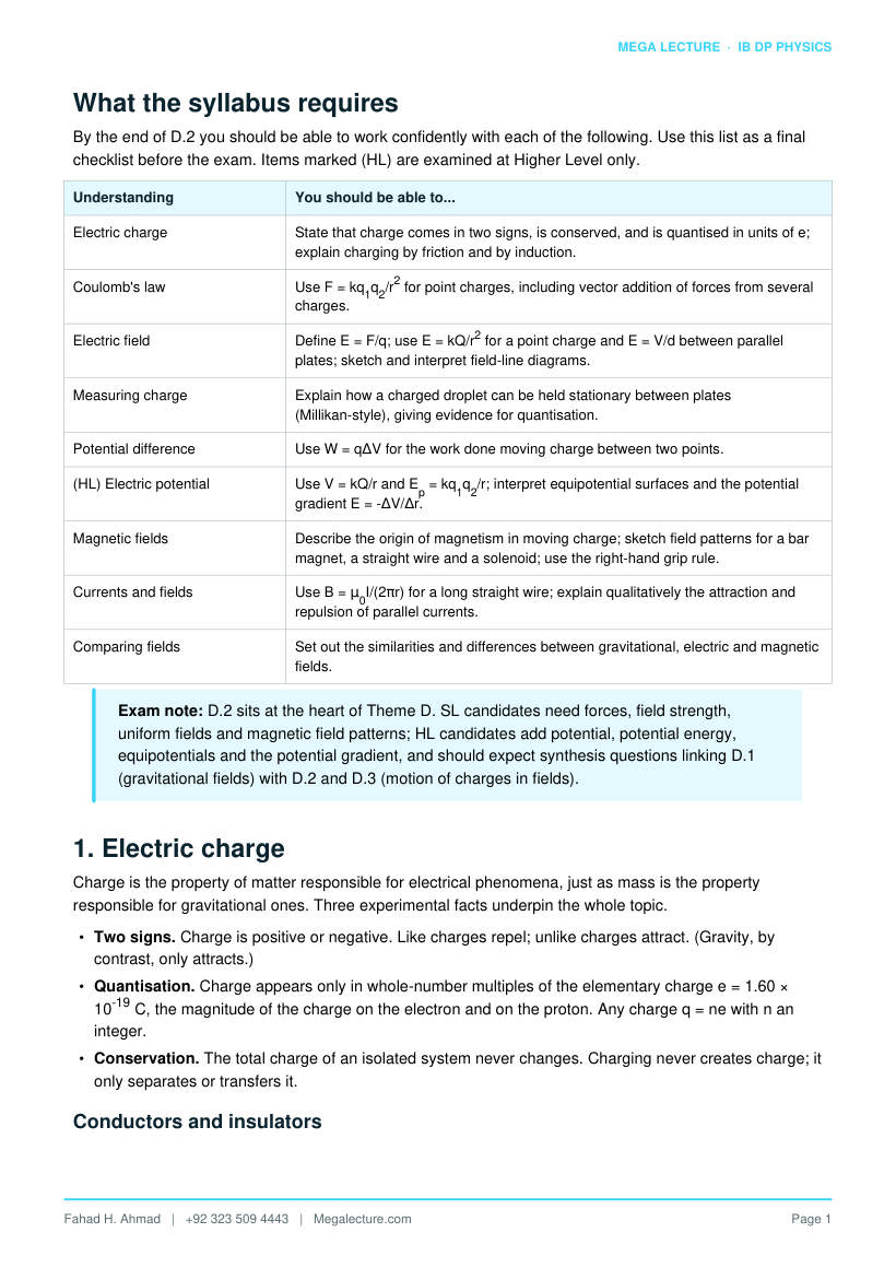
By the end of D.2 you should be able to work confidently with each of the following. Use this list as a final checklist before the exam. Items marked (HL) are examined at Higher Level only.

Understanding You should be able to...

Electric charge State that charge comes in two signs, is conserved, and is quantised in units of e; explain charging by friction and by induction.

Coulomb's law Use F = kq1q2/r2 for point charges, including vector addition of forces from several charges.

Electric field Define E = F/q; use E = kQ/r2 for a point charge and E = V/d between parallel plates; sketch and interpret field-line diagrams.

Measuring charge Explain how a charged droplet can be held stationary between plates (Millikan-style), giving evidence for quantisation.

Potential difference Use W = qΔV for the work done moving charge between two points.

(HL) Electric potential Use V = kQ/r and Ep = kq1q2/r; interpret equipotential surfaces and the potential gradient E = -ΔV/Δr.

Magnetic fields Describe the origin of magnetism in moving charge; sketch field patterns for a bar magnet, a straight wire and a solenoid; use the right-hand grip rule.

Currents and fields Use B = μ0I/(2πr) for a long straight wire; explain qualitatively the attraction and repulsion of parallel currents.

Comparing fields Set out the similarities and differences between gravitational, electric and magnetic fields.

Exam note: D.2 sits at the heart of Theme D. SL candidates need forces, field strength, uniform fields and magnetic field patterns; HL candidates add potential, potential energy, equipotentials and the potential gradient, and should expect synthesis questions linking D.1 (gravitational fields) with D.2 and D.3 (motion of charges in fields).

1. Electric charge

Charge is the property of matter responsible for electrical phenomena, just as mass is the property responsible for gravitational ones. Three experimental facts underpin the whole topic.

• Two signs. Charge is positive or negative. Like charges repel; unlike charges attract. (Gravity, by contrast, only attracts.)
• Quantisation. Charge appears only in whole-number multiples of the elementary charge e = 1.60 × 10-19 C, the magnitude of the charge on the electron and on the proton. Any charge q = ne with n an integer.
• Conservation. The total charge of an isolated system never changes. Charging never creates charge; it only separates or transfers it.

Conductors and insulators

In a conductor (metals, salt solutions, ionised gases) some charges are free to move - in a metal, the delocalised electrons. In an insulator (plastics, glass, dry air) electrons are tightly bound to atoms, so any transferred charge stays where it is put.

Charging by friction and by induction

Friction: rubbing two insulators transfers electrons from one surface to the other. The object that gains electrons becomes negative; the one that loses them becomes equally positive. Only electrons move - a positively charged rod is one that has lost electrons, not gained protons.

Induction: bring a charged rod near (not touching) a conductor and the free electrons shift - attracted toward a positive rod, repelled by a negative one. If the conductor is momentarily earthed while the rod is held in place, electrons flow to or from earth; removing the earth connection and then the rod leaves the conductor with a net charge opposite in sign to the rod. The rod itself loses no charge.

Common misconception: An induced charge is always opposite in sign to the inducing charge, and induction requires no contact. This is also why a charged balloon sticks to a neutral wall: it attracts the opposite induced charges slightly more strongly than it repels the like charges, which are further away.

2. Coulomb's law

Two point charges q1 and q2 a distance r apart exert equal and opposite forces on each other, directed along the line joining them:

F = kq1q2/r2 = q1q2/(4πε0r2) where k = 1/(4πε0) = 8.99 × 109 N m2 C-2 is the Coulomb constant and ε0 = 8.85 × 10-12 C2 N-1 m-2 is the permittivity of free space. The force is an inverse-square law, exactly like Newtonian gravity: doubling r quarters F, so F ∝ 1/r2.

• If the charges have the same sign the product q1q2 is positive and the force is repulsive; opposite signs give attraction.
• In calculations, use magnitudes in the formula and decide the direction physically - safer than juggling signs.
• r is the centre-to-centre separation of the charges, not a gap or a radius. Uniformly charged spheres act as point charges at their centres.
• The law holds for point charges in vacuum (air is an excellent approximation).

Worked example 1 - electric force vs gravity in the hydrogen atom

In a simple model of hydrogen the electron orbits the proton at r = 5.3 × 10-11 m. Compare the electric and gravitational forces between them. (me = 9.11 × 10-31 kg, mp = 1.67 × 10-27 kg)

Electric: FE = ke2/r2 = 8.99 × 109 × (1.60 × 10-19)2 / (5.3 × 10-11)2 = 8.2 × 10-8 N (attractive).

Gravitational: FG = Gmemp/r2 = 6.67 × 10-11 × 9.11 × 10-31 × 1.67 × 10-27 / (5.3 × 10-11)2 = 3.6 × 10-47 N.

Ratio FE/FG ≈ 2 × 1039. This is why gravity is ignored completely in atomic physics, and why bulk matter must be almost exactly neutral - a tiny charge imbalance would swamp gravity.

Forces from several charges: superposition

When more than two charges are present, the resultant force on any one of them is the vector sum of the individual Coulomb forces, each computed pairwise as if the other charges were absent. Forces along a line add with signs; forces at an angle need components or a vector triangle.

Worked example 2 - the null point

Charges of +4.0 μC and +1.0 μC are fixed 0.30 m apart. Where on the line joining them could a third charge rest in equilibrium?

Between the charges, the forces from the two positives on any test charge are opposite in direction; equilibrium requires equal magnitudes. At distance x from the +4.0 μC charge:

k(4.0)/x2 = k(1.0)/(0.30 - x)2

Square-rooting: 2/x = 1/(0.30 - x), so 2(0.30 - x) = x, giving x = 0.20 m from the larger charge (0.10 m from the smaller).

Sense check: the null point always lies closer to the smaller charge, and for two like charges it lies between them. The equilibrium point is the same for any sign of test charge, because both forces scale together.

Exam technique: Never add the magnitudes of forces (or fields) from different charges without first checking directions. Marks are routinely lost by treating vector sums as scalar sums.

3. Electric field

Rather than saying charges act on each other at a distance, we say every charge fills the space around it with an electric field, and other charges respond to the field where they sit. The electric field strength at a point is the force per unit charge on a small positive test charge placed there:

E = F/q (units: N C-1, equivalently V m-1)

E is a vector, pointing in the direction of the force on a positive charge. A negative charge feels a force opposite to E. For a point charge Q, combining the definition with Coulomb's law gives

E = kQ/r2 = Q/(4πε0r2)

Field-line diagrams

Field lines make the field visible. They start on positive charge and end on negative charge (or at infinity); the arrow gives the direction of E; and the density of lines shows the strength - lines crowding together mean a strong field. Field lines never cross, because E has a single direction at each point.

Configuration Pattern to draw

Isolated positive point charge Straight lines radiating symmetrically outward in all directions; spacing grows with distance (inverse-square weakening).

Isolated negative point charge The same radial pattern with every arrow pointing inward.

Dipole (+q and -q) Lines leave the positive charge, curve round and enter the negative charge; densest on the axis between them.

Two equal positive charges Lines repel each other; a neutral (null) point with zero field lies midway between the charges, where no line passes.

Oppositely charged parallel plates

Straight, equally spaced parallel lines from + plate to - plate: a uniform field. Lines bulge outward slightly at the edges, where the field weakens.

Figure 1. Left: the field of a single positive charge points radially outward. Middle: the dipole field runs from the + charge to the

− charge. Right: the Coulomb force F = kq1q2/r2 ∝ 1/r2, so doubling r quarters F (0.10 N to 0.025 N).

Worked example 3 - adding fields as vectors

Charges +3.0 μC and -3.0 μC are held 0.40 m apart. Find the electric field at the midpoint of the line joining them.

Each charge is r = 0.20 m from the midpoint, so each contributes

E = kQ/r2 = 8.99 × 109 × 3.0 × 10-6 / 0.202 = 6.7 × 105 N C-1

The field of the positive charge points away from it (toward the negative charge); the field of the negative charge points toward itself - the same direction. The two contributions add:

Etotal = 2 × 6.7 × 105 ≈ 1.3 × 106 N C-1, directed from + to -.

Contrast: at the midpoint of two equal positive charges the two fields are equal and opposite and the resultant is zero.

The uniform field between parallel plates

Two parallel plates with a potential difference V across them and a separation d produce a uniform field in the gap:

E = V/d

Uniform means E has the same magnitude and direction everywhere between the plates (away from the edges), pointing from the positive plate to the negative plate. A charge q in the gap feels a constant force F = qE = qV/d, so it accelerates uniformly - the electrical analogue of projectile motion, treated fully in D.3.

Worked example 4 - electron between plates

Two plates 8.0 mm apart have a potential difference of 400 V. Find the field strength, and the force on and acceleration of an electron in the gap.

E = V/d = 400 / 8.0 × 10-3 = 5.0 × 104 V m-1

F = eE = 1.60 × 10-19 × 5.0 × 104 = 8.0 × 10-15 N, directed toward the positive plate (opposite to E, since the electron is negative).

a = F/m = 8.0 × 10-15 / 9.11 × 10-31 ≈ 8.8 × 1015 m s-2 - about 1015 times g, so gravity on the electron is utterly negligible.

Figure 3. The uniform field between parallel plates: equally spaced parallel lines run from the + plate to the − plate. With V =

400 V across d = 8.0 mm, E = V/d = 5.0×104 V m-1.

4. Weighing a charge: the Millikan idea

A uniform field can hold a charged object stationary against gravity. This is the principle of Millikan's oil-drop experiment, the classic evidence that charge is quantised. A tiny charged droplet between horizontal plates is in equilibrium when the upward electric force balances its weight:

qE = mg so q = mgd/V

Millikan measured q for hundreds of droplets and found every value was a whole multiple of 1.6 × 10-19 C - never a fraction of it. That integer staircase is the experimental meaning of quantisation.

Worked example 5 - balancing a droplet

An oil droplet of mass 3.2 × 10-15 kg is held stationary between plates 5.0 mm apart when the potential difference is 490 V. Find the charge on the droplet and the number of elementary charges it carries. (g = 9.8 m s-2)

E = V/d = 490 / 5.0 × 10-3 = 9.8 × 104 V m-1 qE = mg gives q = mg/E = 3.2 × 10-15 × 9.8 / 9.8 × 104 = 3.2 × 10-19 C n = q/e = 3.2 × 10-19 / 1.6 × 10-19 = 2 elementary charges. For the force to be upward, the droplet must carry charge of the sign attracted to the upper plate - here two surplus electrons if the upper plate is positive.

Exam technique: Balance questions are force diagrams in disguise: weight mg down, electric force qE up, in equilibrium. If the droplet instead moves at constant velocity, drag joins the diagram but the resultant is still zero.

5. Electric potential difference and potential

The potential difference (p.d.) ΔV between two points is the work done per unit charge in moving a small positive test charge between them:

W = qΔV (1 volt = 1 joule per coulomb)

This is the workhorse energy equation of electricity. A charge q accelerated from rest through a p.d. V gains kinetic energy qV; a charge pushed the "wrong way" against the field requires work qV from an external agent. It also defines the electronvolt: 1 eV = 1.60 × 10-19 J, the energy gained by one elementary charge crossing one volt.

Worked example 6 - accelerating an electron

An electron is accelerated from rest through a potential difference of 5.0 kV in an X-ray tube. Find its kinetic energy and final speed.

W = qΔV = 1.60 × 10-19 × 5.0 × 103 = 8.0 × 10-16 J (= 5.0 keV)

½mv2 = 8.0 × 10-16 J gives v = (2 × 8.0 × 10-16 / 9.11 × 10-31)1/2 ≈ 4.2 × 107 m s-1

That is 14% of the speed of light - fast enough that a relativistic treatment (A.5) would start to matter at slightly higher voltages.

(HL) Electric potential of a point charge

The electric potential V at a point is the work done per unit charge in bringing a small positive test charge from infinity to that point. Potential is a scalar: contributions from several charges add algebraically, signs included, with no components to resolve. For a point charge Q:

V = kQ/r = Q/(4πε0r)

Note 1/r, not 1/r2. V is positive near positive charge, negative near negative charge, and zero at infinity by convention. The potential energy of two point charges follows directly:

Ep = kq1q2/r

Ep is positive for like charges (work had to be done pushing them together) and negative for unlike charges (they are bound; work is needed to separate them).

Worked example 7 (HL) - potential and potential energy

A point charge Q = -3.0 nC is fixed in place. (a) Find the potential 0.12 m from it. (b) Find the electric potential energy of a +2.0 nC charge placed at that point. (c) How much work is needed to drag the +2.0 nC charge away to infinity?

• V = kQ/r = 8.99 × 109 × (-3.0 × 10-9) / 0.12 = -225 V (≈ -220 V to 2 s.f.)
• Ep = qV = 2.0 × 10-9 × (-225) = -4.5 × 10-7 J. The negative sign says the pair is bound.
• W = Ep(infinity) - Ep(r) = 0 - (-4.5 × 10-7) = +4.5 × 10-7 J of work must be supplied.

(HL) Equipotentials and the potential gradient

An equipotential surface joins points at the same potential. Moving a charge anywhere along an equipotential takes zero work (W = qΔV and ΔV = 0), so field lines always cross equipotentials at right angles. Around a point charge the equipotentials are concentric spheres; between parallel plates they are planes parallel to the plates; equipotentials drawn at equal voltage steps crowd together where the field is strong.

The field is the negative gradient of the potential:

E = -ΔV/Δr

The minus sign records that E points from high potential to low potential - "downhill". A positive charge released from rest accelerates toward lower potential; a negative charge toward higher potential. On a graph of V against r, the field strength is minus the gradient; on a graph of E against r, the area under the curve gives the change in potential.

Gravity and electricity: one mathematics, two forces

Examiners love asking for parallels between D.1 and D.2. The mathematics is identical; only the constant, the property and the possibility of repulsion change.

Gravitational (D.1) Electric (D.2)

Acts on mass m charge q

Force law F = Gm1m2/r2 F = kq1q2/r2

Field strength g = F/m = GM/r2 E = F/q = kQ/r2

Potential (HL) Vg = -GM/r (always negative) Ve = kQ/r (either sign)

Potential energy (HL) Ep = -Gm1m2/r Ep = kq1q2/r

Gravitational (D.1) Electric (D.2)

Field from potential (HL) g = -ΔVg/Δr E = -ΔVe/Δr

Direction of force Always attractive Attractive or repulsive

Relative strength Extremely weak Stronger by ≈ 1039 (hydrogen atom)

Shielding possible? No Yes - conductors screen electric fields

HL exam favourite: "State one similarity and one difference between the electric field of a point charge and the gravitational field of a point mass." Similarity: both are radial inverse-square fields. Difference: gravitational forces are only attractive, electric forces can be repulsive (equivalently: only one sign of mass exists).

6. Magnetic fields

Magnetism is not a separate phenomenon from electricity: all magnetic fields originate in moving charge - currents in wires, orbiting and spinning electrons in atoms. In a permanent magnet the atomic current loops of many electrons are aligned so their fields add; in an unmagnetised material they point randomly and cancel. There is no magnetic equivalent of charge: no magnetic monopoles have ever been observed. North and south poles always come in pairs - cutting a bar magnet in half yields two smaller complete magnets, not separated poles.

Magnetic field lines

The magnetic field B is a vector field mapped by field lines, with direction defined as the direction in which the north pole of a small compass points. Because there are no monopoles, magnetic field lines never start or stop: they form closed loops.

Source Field pattern

Bar magnet Loops emerging from the north pole, curving round to enter the south pole, continuing inside the magnet from S back to N. Densest at the poles, where the field is strongest.

Long straight current-carrying wire

Concentric circles centred on the wire, in planes perpendicular to it. Direction from the right-hand grip rule: thumb along the conventional current, fingers curl the way the field circulates. Circles space out with distance as the field weakens.

Solenoid (long coil) Inside: strong, uniform, straight lines parallel to the axis. Outside: the field of a bar magnet, with one end acting as N and the other as S. Grip rule for coils: curl the fingers with the current, the thumb gives N.

The Earth Approximately the field of a bar magnet tilted from the spin axis, with the magnetic pole in the northern hemisphere being a magnetic south pole (it attracts compass north poles). Surface field strength of order 10-5 T.

Two like poles repel and unlike poles attract, but unlike the electric case there is no simple pole-strength formula on the syllabus: magnetic field calculations start from currents.

Common misconception: Field lines inside the magnet run from S to N, completing the loop - they do not stop at the poles. Diagrams that show lines beginning and ending on a magnet lose marks at HL.

7. Magnetic fields from currents

Field of a long straight wire

At perpendicular distance r from a long straight wire carrying current I,

B = μ0I/(2πr) where μ0 = 4π × 10-7 T m A-1 is the permeability of free space. The field strength falls as 1/r (not inverse-square: the source is a line, not a point), and B ∝ I. The unit of B is the tesla, T = N A-1 m-1: one tesla is a very strong field (an MRI magnet is a few T; a fridge magnet about 10-2 T).

Worked example 8 - field near a wire

A long straight wire carries a current of 5.0 A. Find the magnetic field strength 2.0 cm from the wire, and compare it with the Earth's field (≈ 5 × 10-5 T).

B = μ0I/(2πr) = (4π × 10-7 × 5.0) / (2π × 0.020) = 2 × 10-7 × 5.0 / 0.020 = 5.0 × 10-5 T

This equals the Earth's field - which is why a compass held near household wiring carrying a few amps visibly deflects, and why Oersted's compass experiment of 1820 could reveal electromagnetism with such simple apparatus.

Figure 2. The magnetic field of a long straight wire carrying current I out of the page: concentric circles given by B = μ0I/(2πr).

At r = 2.0 cm with I = 5.0 A, B = 5.0×10-5 T, comparable to the Earth's field.

Solenoid

Stacking many turns of wire multiplies the effect: inside a long solenoid the field is strong and uniform, proportional to the current and to the number of turns per unit length, and essentially independent of position (a treatment kept qualitative at this level). An iron core strengthens the field enormously - the electromagnet. The uniform interior field is the magnetic analogue of the uniform electric field between parallel plates.

Force between parallel currents

Each wire sits in the magnetic field of the other, so each experiences a force (the current-in-a-field force F = BIL is developed in D.3, but the logic belongs here):

• Currents in the same direction attract.
• Currents in opposite directions repel.

The force per unit length on each of two long parallel wires distance d apart is

F/L = μ0I1I2/(2πd)

The forces on the two wires are equal and opposite (Newton's third law) even when the currents differ. This mutual force was the basis of the pre-2019 definition of the ampere: the current which, flowing in two long parallel wires one metre apart in vacuum, produces a force of exactly 2 × 10-7 N per metre of wire. (The ampere is now defined by fixing the numerical value of e.)

Worked example 9 - parallel wires

Two long parallel wires 5.0 cm apart each carry 3.0 A in the same direction. Find the force per unit length between them and state its nature.

F/L = μ0I1I2/(2πd) = 2 × 10-7 × (3.0 × 3.0) / 0.050 = 3.6 × 10-5 N m-1, attractive.

Direction logic: wire 1 creates circles of field around itself; at wire 2 this field is perpendicular to wire 2's current, producing a force directed back toward wire 1. Repeat the argument from wire 2 and the forces point toward each other: attraction.

Common misconception: "Same currents attract" is the opposite of the charge rule ("like charges repel"). Do not let the electrostatic instinct leak into the magnetic case.