Costs of production: fixed, variable, average and marginal costs, short run and long run

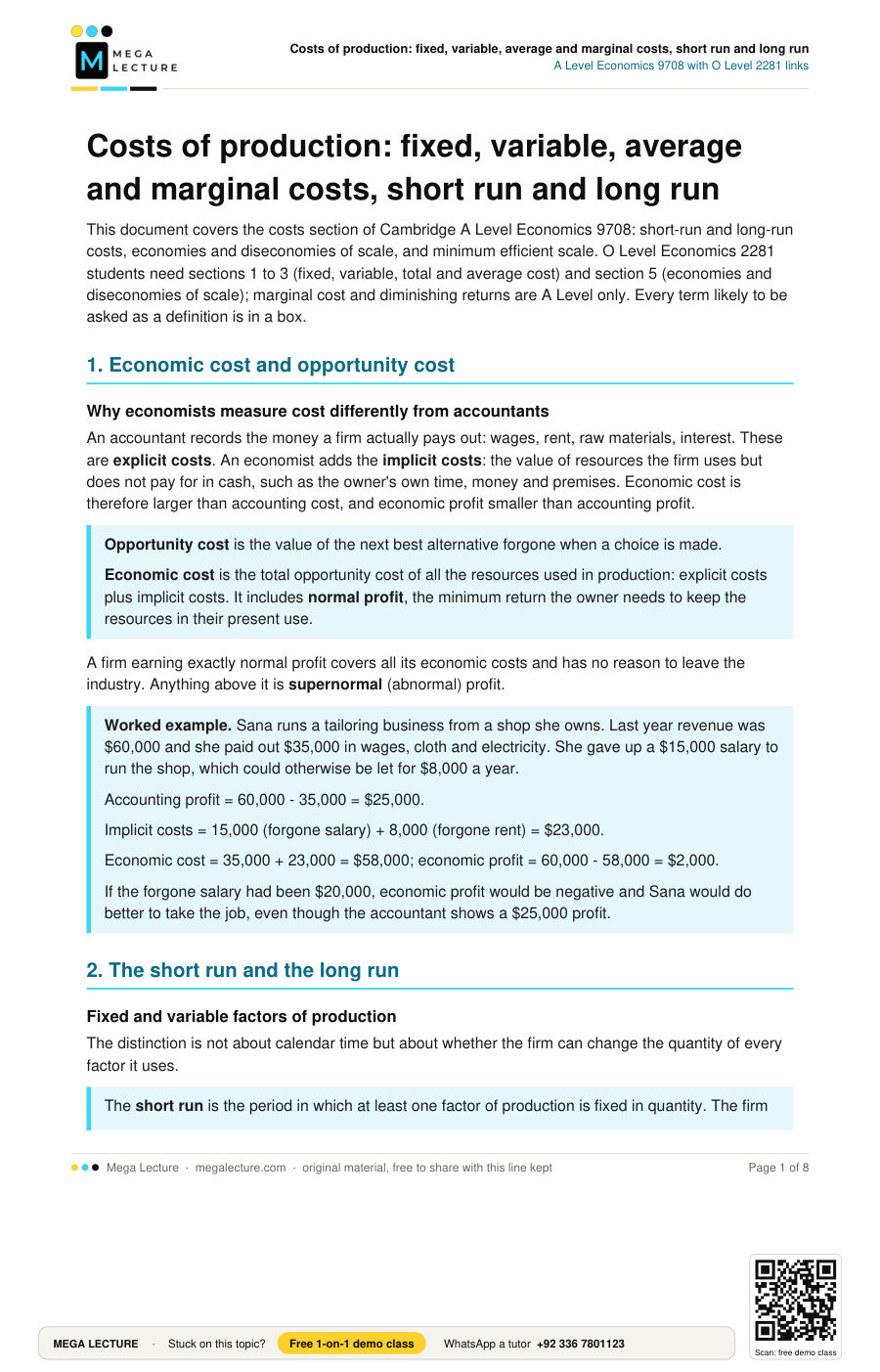
This document covers the costs section of Cambridge A Level Economics 9708: short-run and long-run costs, economies and diseconomies of scale, and minimum efficient scale. O Level Economics 2281 students need sections 1 to 3 (fixed, variable, total and average cost) and section 5 (economies and diseconomies of scale); marginal cost and diminishing returns are A Level only. Every term likely to be asked as a definition is in a box.

1. Economic cost and opportunity cost

Why economists measure cost differently from accountants

An accountant records the money a firm actually pays out: wages, rent, raw materials, interest. These are explicit costs. An economist adds the implicit costs: the value of resources the firm uses but does not pay for in cash, such as the owner's own time, money and premises. Economic cost is therefore larger than accounting cost, and economic profit smaller than accounting profit.

Opportunity cost is the value of the next best alternative forgone when a choice is made.

Economic cost is the total opportunity cost of all the resources used in production: explicit costs plus implicit costs. It includes normal profit, the minimum return the owner needs to keep the resources in their present use.

A firm earning exactly normal profit covers all its economic costs and has no reason to leave the industry. Anything above it is supernormal (abnormal) profit.

Worked example. Sana runs a tailoring business from a shop she owns. Last year revenue was $60,000 and she paid out $35,000 in wages, cloth and electricity. She gave up a $15,000 salary to run the shop, which could otherwise be let for $8,000 a year.

Accounting profit = 60,000 - 35,000 = $25,000.

Implicit costs = 15,000 (forgone salary) + 8,000 (forgone rent) = $23,000.

Economic cost = 35,000 + 23,000 = $58,000; economic profit = 60,000 - 58,000 = $2,000.

If the forgone salary had been $20,000, economic profit would be negative and Sana would do better to take the job, even though the accountant shows a $25,000 profit.

2. The short run and the long run

Fixed and variable factors of production

The distinction is not about calendar time but about whether the firm can change the quantity of every factor it uses.

The short run is the period in which at least one factor of production is fixed in quantity. The firm can change output only by changing its variable factors, usually labour and raw materials.

The long run is the period in which all factors of production are variable. The firm can change the size of its plant and so its scale of production.

A food stall's short run lasts weeks; a steel maker's lasts years. In the long run there are no fixed costs.

3. Fixed, variable, total, average and marginal cost

Total costs

Fixed costs (total fixed cost, TFC) are costs that do not change with the level of output in the short run: rent, insurance, interest on a loan, a manager's salary. They must be paid even when output is zero.

Variable costs (total variable cost, TVC) are costs that change directly with the level of output: raw materials, electricity used by machines, wages of workers paid by the hour or by the piece.

Total cost (TC) is the sum of fixed and variable costs: TC = TFC + TVC.

Average costs

Average fixed cost (AFC) = TFC ÷ output (Q).

Average variable cost (AVC) = TVC ÷ Q.

Average total cost (AC or ATC) = TC ÷ Q. Because TC = TFC + TVC, AC = AFC + AVC.

Marginal cost

Marginal cost (MC) is the addition to total cost from producing one more unit of output: MC = change in TC ÷ change in Q.

Because fixed costs do not change when output changes, MC can equally be found from the change in variable cost: MC = change in TVC ÷ change in Q.

A worked cost table

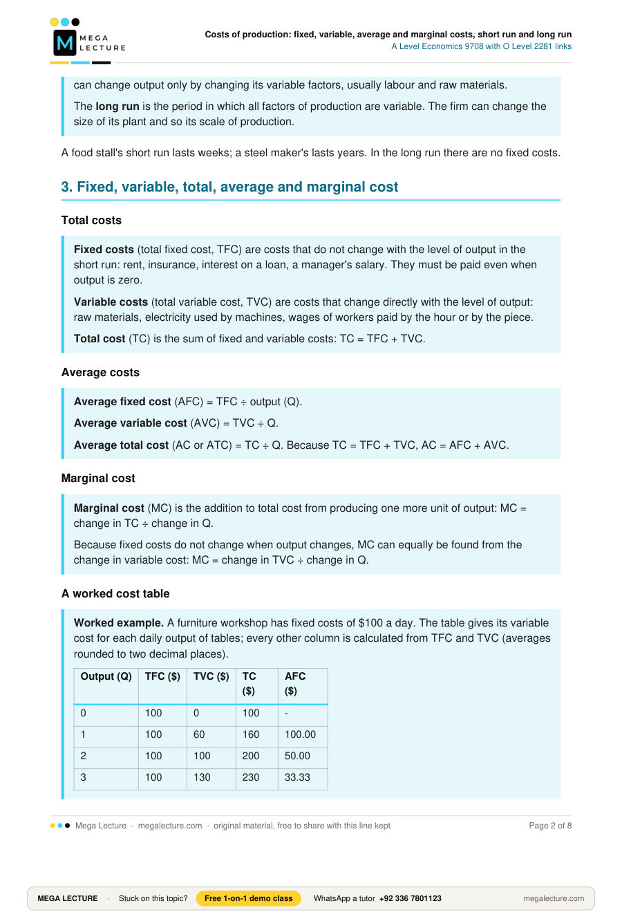
Worked example. A furniture workshop has fixed costs of $100 a day. The table gives its variable cost for each daily output of tables; every other column is calculated from TFC and TVC (averages rounded to two decimal places).

Output (Q)	TFC ($)	TVC ($)	TC ($)	AFC ($)	AVC ($)	AC ($)	MC ($)
0	100	0	100	-	-	-	-
1	100	60	160	100.00	60.00	160.00	60
2	100	100	200	50.00	50.00	100.00	40
3	100	130	230	33.33	43.33	76.67	30
4	100	170	270	25.00	42.50	67.50	40
5	100	230	330	20.00	46.00	66.00	60
6	100	310	410	16.67	51.67	68.33	80
7	100	410	510	14.29	58.57	72.86	100
8	100	530	630	12.50	66.25	78.75	120

How each column was found, using Q = 3: TC = 100 + 130 = 230; AFC = 100 ÷ 3 = 33.33; AVC = 130 ÷ 3 = 43.33; AC = 230 ÷ 3 = 76.67 (also 33.33 + 43.33); MC = 230 - 200 = 30, the extra cost of the third table.

Four things to notice, each a standard exam point:

1. TFC is the same at every output, including zero, so at zero output TC = TFC.
2. AFC never stops falling, because the same $100 is spread over more tables.
3. MC falls at first (60, 40, 30) and then rises (40, 60, 80, 100, 120); the turning point is where diminishing returns set in (section 4).
4. AVC is lowest at Q = 4 ($42.50) and AC at Q = 5 ($66.00): the falling AFC keeps pulling AC down a little longer. Wherever MC is below AC, AC is falling (Q = 1 to 5); wherever MC is above AC, AC is rising (Q = 6 onwards). MC crosses AC at AC's minimum, between Q = 5 and Q = 6.

4. The law of diminishing returns and the shape of the short-run cost curves

The law of diminishing returns

The law of diminishing returns (the law of diminishing marginal returns, or of variable proportions) states that as more units of a variable factor are added to a fixed factor, there comes a point beyond which each additional unit of the variable factor adds less to total output than the previous unit did: marginal product falls.

The law needs a fixed factor, so it is a short-run law. In a kitchen of fixed size the first few cooks can specialise, so marginal product rises; beyond some number extra cooks get in each other's way, and each adds less than the one before.

From returns to costs

If each worker is paid the same wage W and adds MP units of output, the extra cost per extra unit is MC = W ÷ MP. While marginal product rises, MC falls; once marginal product falls, MC rises. This gives the MC curve its tick shape. In the worked table, diminishing returns set in at the fourth table, where MC turns up.

The shapes of AFC, AVC and AC

• AFC falls continuously towards zero: a rectangular hyperbola.
• AVC is U-shaped: it falls while marginal product rises and rises once diminishing returns take hold.
• AC is U-shaped and lies above AVC; the gap between them is AFC, so it narrows as output rises. AC turns up after AVC does.
• MC reaches its minimum first, then rises and cuts AVC and AC at their minimum points.

Why MC cuts AC at the minimum of AC

This is the relationship between any marginal and any average. A batsman averaging 40 who scores 20 in his next innings sees his average fall; if he scores 60 it rises. The same logic applies to cost:

If MC is below AC, producing one more unit adds less than the current average, so AC falls.

If MC is above AC, producing one more unit adds more than the current average, so AC rises.

AC can therefore only stop falling and start rising at the output where MC = AC, which is the minimum point of AC. The same argument shows that MC cuts AVC at the minimum of AVC.

In the worked table: at Q = 5, MC (60) is below AC (66) and AC is still falling; at Q = 6, MC (80) is above AC (68.33) and AC is rising. The curves cross between these outputs.

5. Long-run costs: economies and diseconomies of scale

Returns to scale are not diminishing returns

In the long run there is no fixed factor, so the law of diminishing returns does not apply. Instead the firm changes its scale, the amount of every factor. If doubling all inputs more than doubles output, long-run average cost falls: economies of scale. If doubling all inputs less than doubles output, long-run average cost rises: diseconomies of scale. Keep the ideas apart: diminishing returns is short run with one factor fixed; economies and diseconomies of scale are long run with all factors changing.

Economies of scale are the reductions in long-run average cost that a firm gains as it increases its scale of production.

Diseconomies of scale are the increases in long-run average cost that a firm experiences when it grows beyond a certain size.

Internal economies and diseconomies arise from the growth of the firm itself. External economies and diseconomies arise from the growth of the industry the firm is in, and affect all the firms in that industry whatever their individual size.

Internal economies of scale

• Technical economies. Large firms can use large, indivisible machines (an assembly line is no use at half size) that are cheapest per unit at full capacity. The container principle: a tank with double the dimensions holds eight times as much but needs only four times the material. Large output also allows division of labour.
• Purchasing (bulk-buying) economies. Large orders earn a lower price per unit from suppliers.
• Marketing economies. An advertising campaign costs much the same whether the firm sells 10,000 or 1,000,000 units, so cost per unit falls as output rises.
• Financial economies. Large firms are seen as lower risk and borrow at lower interest rates; they can also issue shares.
• Managerial economies. A large firm can afford specialist managers (accountant, human resources, logistics) whose expertise lowers cost per unit.
• Risk-bearing economies. A large firm can sell a range of products in several markets, so a fall in one market does not threaten the whole firm.

Internal diseconomies of scale

• Communication problems. Messages pass through many layers of management, so they are slower and distorted and decisions are delayed.
• Co-ordination problems. It is harder to monitor many plants and departments, so waste goes unnoticed and more managers are needed to manage other managers.
• Motivation problems. Workers in a huge organisation may feel like a small cog, so productivity falls and absenteeism rises.

External economies and diseconomies of scale

External economies lower the average cost of every firm in an industry when the industry grows or concentrates in one area: a local pool of skilled workers develops, colleges run relevant courses, specialist suppliers set up nearby, transport improves, and firms share research through trade associations. Textile firms in Faisalabad enjoy these benefits.

External diseconomies raise the average cost of every firm when the industry grows too large for its area: roads become congested, firms bid up wages for the same skilled workers, rents rise, and raw materials become scarcer and dearer.

The long-run average cost curve

Each plant size has its own short-run average cost curve. The long-run average cost (LRAC) curve is the envelope of all of them: the lowest average cost at which each output can be produced once the firm has chosen the best plant size. LRAC falls at first (economies of scale), may be flat over a range (constant returns to scale), and eventually rises (diseconomies of scale). In many industries it looks more like an L than a U, because firms find ways to avoid diseconomies.

6. Minimum efficient scale

The minimum efficient scale (MES) is the lowest level of output at which long-run average cost reaches its minimum, that is, the output at which a firm has gained all the available economies of scale.

MES shapes the structure of an industry:

• MES small relative to market demand (hairdressing, restaurants): many firms can each reach minimum cost, so the industry has many small firms.
• MES large relative to market demand (aircraft, steel): only a few firms can reach it, so the industry becomes an oligopoly.
• MES so large that one firm can supply the whole market more cheaply than two could: a natural monopoly (water supply, electricity transmission).

A high MES is also a barrier to entry: a new firm would need to enter at a very large scale to match the costs of existing firms.

7. Worked calculation set

Calculation 1: costs from a total cost schedule. A firm's total cost is $500 at zero output, $800 at 10 units, $1,000 at 20 units, $1,300 at 30 units and $1,800 at 40 units.

TFC = $500 (total cost at zero output). TVC at 30 units = 1,300 - 500 = $800, so AVC at 30 = 800 ÷ 30 = $26.67.

AC at 20 = 1,000 ÷ 20 = $50; AC at 30 = 1,300 ÷ 30 = $43.33; AC at 40 = 1,800 ÷ 40 = $45.

MC per unit between 30 and 40 = (1,800 - 1,300) ÷ 10 = $50, above AC at 30 ($43.33), so AC rises between 30 and 40, as the figures confirm.

Calculation 2: constant marginal cost. A printer's total cost is TC = 2,000 + 5Q, where Q is the number of books printed.

TFC = $2,000 and MC = $5 for every book (the coefficient of Q).

AC at Q = 100: (2,000 + 500) ÷ 100 = $25. AC at Q = 1,000: (2,000 + 5,000) ÷ 1,000 = $7. AC at Q = 10,000: 52,000 ÷ 10,000 = $5.20.

AC falls continuously and approaches $5 but never reaches it: MC ($5) is always below AC, so AC keeps falling. There are no diminishing returns here because MC never rises.

Quick check

1. Define opportunity cost. [2]
2. Explain the difference between the accounting cost and the economic cost of running a business. [4]
3. State whether each of the following is a fixed cost or a variable cost for a bakery: (a) the monthly rent of the shop, (b) flour, (c) the annual insurance premium, (d) the electricity used by the ovens. [4]
4. A firm has fixed costs of $200. Its total variable costs are $150 at 1 unit, $250 at 2 units, $330 at 3 units, $450 at 4 units and $650 at 5 units. Calculate total cost, average fixed cost, average variable cost, average cost and marginal cost at each output, and state the output at which average cost is lowest. [8]
5. A firm's average cost at 10 units is $50. The marginal cost of the 11th unit is $72. Calculate the average cost at 11 units and explain why it has changed in the direction it has. [3]
6. Explain why the marginal cost curve cuts the average cost curve at the minimum point of the average cost curve. [4]
7. State the law of diminishing returns and explain why it applies only in the short run. [4]
8. Explain how the law of diminishing returns causes the marginal cost curve to rise. [3]
9. Distinguish between internal and external economies of scale, giving one example of each. [4]
10. Define minimum efficient scale and explain how it influences the number of firms in an industry. [4]
11. "A firm should always increase its scale of production, because it will gain economies of scale." Evaluate this statement. [6]

1. Opportunity cost is the value of the next best alternative forgone (1) when a choice is made or a resource is used for one purpose rather than another (1).

2. Accounting cost is the total of explicit costs, the money actually paid out for wages, materials, rent and so on (1). Economic cost adds the implicit costs, the opportunity cost of resources the owner supplies without a cash payment, such as a forgone salary or forgone rent (1). It also includes normal profit, the minimum return needed to keep the owner in the industry (1). Economic cost is therefore higher, so a firm showing an accounting profit may be making an economic loss (1).

3. (a) Fixed: rent must be paid whatever the output. (b) Variable: more bread needs more flour. (c) Fixed: the premium does not depend on how much is baked. (d) Variable: the ovens use more electricity when more is baked. (1 mark each)

4. TC = 200 + TVC; AFC = 200 ÷ Q; AVC = TVC ÷ Q; AC = TC ÷ Q; MC = change in TC.

Q	TC ($)	AFC ($)	AVC ($)	AC ($)	MC ($)
1	350	200.00	150.00	350.00	150
2	450	100.00	125.00	225.00	100
3	530	66.67	110.00	176.67	80
4	650	50.00	112.50	162.50	120
5	850	40.00	130.00	170.00	200

Average cost is lowest at 4 units ($162.50). Check with the average-marginal rule: the MC of the 4th unit ($120) is below AC, so AC was still falling; the MC of the 5th unit ($200) is above AC, so AC rises. (TC 2, AFC 1, AVC 1, AC 2, MC 1, lowest AC 1)

5. TC at 10 units = 10 × 50 = $500. TC at 11 units = 500 + 72 = $572. AC at 11 = 572 ÷ 11 = $52 (2). AC has risen because the marginal cost of the extra unit ($72) was greater than the average cost ($50), so it pulls the average up (1).

6. Marginal cost is the cost of the last unit; average cost is the cost per unit over all units (1). When MC is below AC, the last unit costs less than the average, so adding it pulls the average down and AC falls (1). When MC is above AC, the last unit costs more than the average and AC rises (1). AC can only change from falling to rising at the output where MC = AC, which is therefore the minimum point of AC (1).

7. The law of diminishing returns states that when increasing quantities of a variable factor are added to a fixed factor, there comes a point after which each extra unit of the variable factor adds less to total output than the one before, so marginal product falls (2). It applies only in the short run because it depends on there being a fixed factor (1). In the long run all factors are variable, so the firm can increase everything in proportion and the constraint disappears; long-run changes in cost come from economies and diseconomies of scale instead (1).

8. Marginal cost equals the wage divided by the marginal product of labour, MC = W ÷ MP (1). Once diminishing returns set in, marginal product falls, so each extra worker adds fewer units of output (1). The same wage is spread over fewer extra units, so the cost of each extra unit, MC, rises (1).

9. Internal economies of scale are falls in long-run average cost that result from the growth of the firm itself and are available only to that firm (1); example: bulk-buying discounts, a large indivisible machine, or cheaper borrowing (1). External economies of scale are falls in average cost that result from the growth of the whole industry or its concentration in one area and benefit all the firms in it regardless of their own size (1); example: a local pool of skilled labour, specialist suppliers nearby, or better transport links (1).

10. Minimum efficient scale is the lowest output at which a firm's long-run average cost reaches its minimum, the point where all economies of scale have been gained (2). If MES is small compared with market demand, many firms can each produce at minimum cost, so the industry contains many firms (1). If MES is large compared with the market, only a few firms can reach it, so the industry is dominated by a few large firms, or by a natural monopoly if one firm's MES is as large as the whole market; a high MES also deters new entrants (1).

11. For: a larger scale can lower long-run average cost through technical, purchasing, financial and marketing economies, allowing lower prices or higher margins (up to 3). Against: economies of scale run out at the minimum efficient scale, and beyond some size diseconomies set in as communication slows and co-ordination and motivation weaken, so average cost rises (1). Expansion also depends on demand: producing more than the firm can sell gains nothing (1). Judgement: the statement is too strong; a firm should expand only up to the output where long-run average cost stops falling, and only when demand justifies it (1 for a supported conclusion).